0. set up

Code

# cleaning
library(tidyverse)

# visualization
library(showtext)
font_add_google("Lato", "Lato")

1. anemone regression example

Code

# number of anemones in a clump
clump <- seq(from = 1, to = 60, by = 1)

# circumference: anemones can be up to 8 cm long
set.seed(10)
circ <- rnorm(length(clump), mean = seq(from = 1, to = 5, length = length(clump)), sd = 1) 

# create a data frame
df <- cbind(circ, clump) %>% 
  as.data.frame() 

# linear model
lm(circ ~ clump, data = df) %>% summary()


Call:
lm(formula = circ ~ clump, data = df)

Residuals:
     Min       1Q   Median       3Q      Max 
-1.88621 -0.62425  0.06147  0.58350  2.17217 

Coefficients:
            Estimate Std. Error t value Pr(>|t|)    
(Intercept) 0.451168   0.236422   1.908   0.0613 .  
clump       0.076068   0.006741  11.285 2.91e-16 ***
---
Signif. codes:  0 '***' 0.001 '**' 0.01 '*' 0.05 '.' 0.1 ' ' 1

Residual standard error: 0.9042 on 58 degrees of freedom
Multiple R-squared:  0.6871,    Adjusted R-squared:  0.6817 
F-statistic: 127.3 on 1 and 58 DF,  p-value: 2.914e-16

Code

showtext_auto()
ggplot(df, aes(x = clump, y = circ)) +
  geom_point(size = 2) +
  # just using geom smooth for the purposes of visualization
  geom_smooth(method = "lm", se = FALSE, linewidth = 2) +
  labs(x = "Number of anemones in a colony", y = "Circumference (cm)") +
  theme_bw() +
  theme(panel.grid = element_blank(),
        axis.text = element_text(size = 18),
        axis.title = element_text(size = 18),
        text = element_text(family = "Lato"))

`geom_smooth()` using formula = 'y ~ x'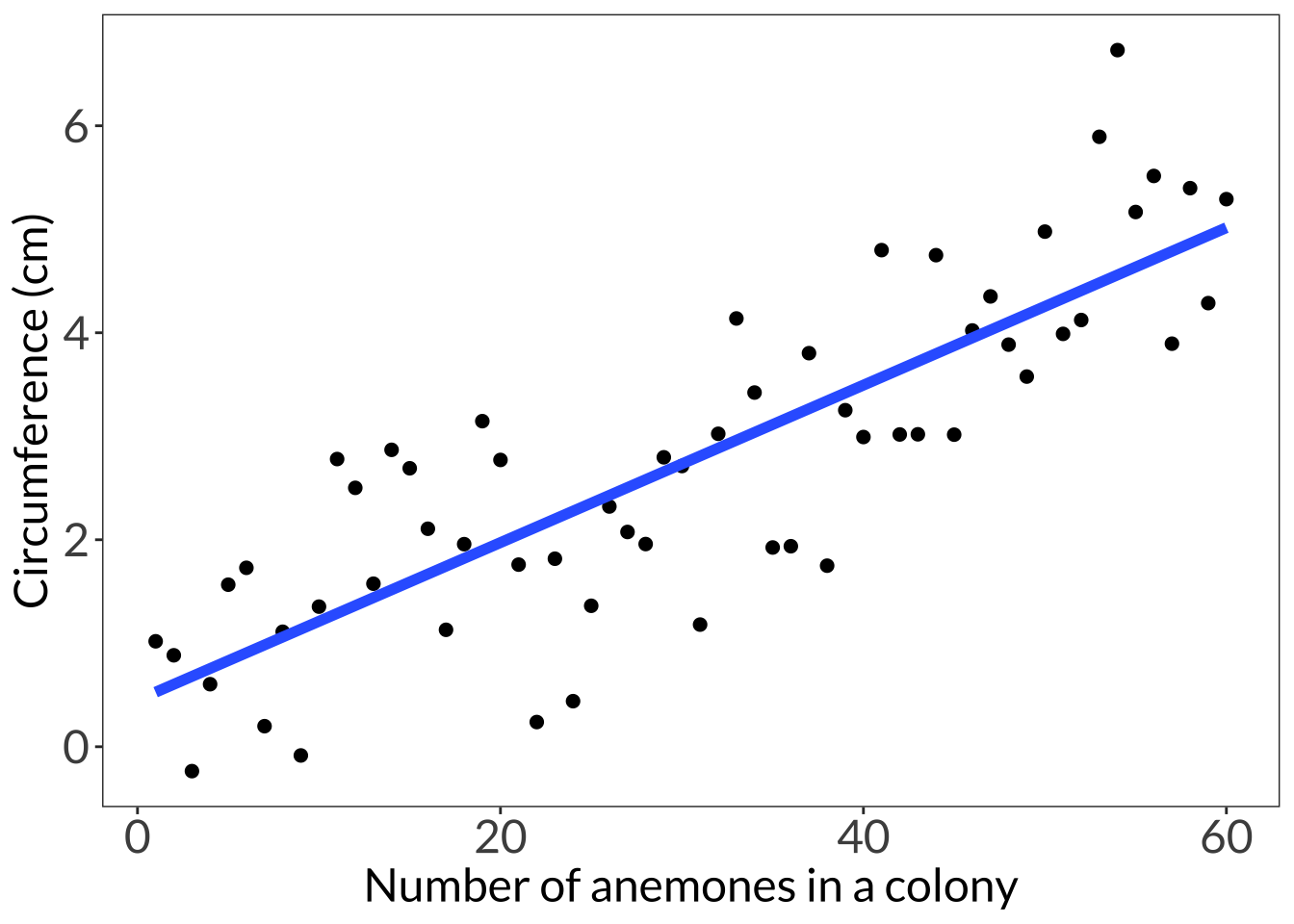

2. histogram example

Code

ggplot(df, aes(x = circ)) +
  scale_x_continuous(breaks = seq(from = 0, to = 7, by = 1)) +
  scale_y_continuous(expand = c(0, 0), limits = c(0, 19), breaks = seq(from = 0, to = 18, by = 3)) +
  geom_histogram(breaks = seq(from = 0, to = 7, by = 1), color = "#000000", fill = "lightblue") +
  labs(x = "Anemone circumference (cm)", y = "Count") +
  theme_bw() +
  theme(panel.grid = element_blank(),
        axis.text = element_text(size = 18),
        axis.title = element_text(size = 18),
        text = element_text(family = "Lato"))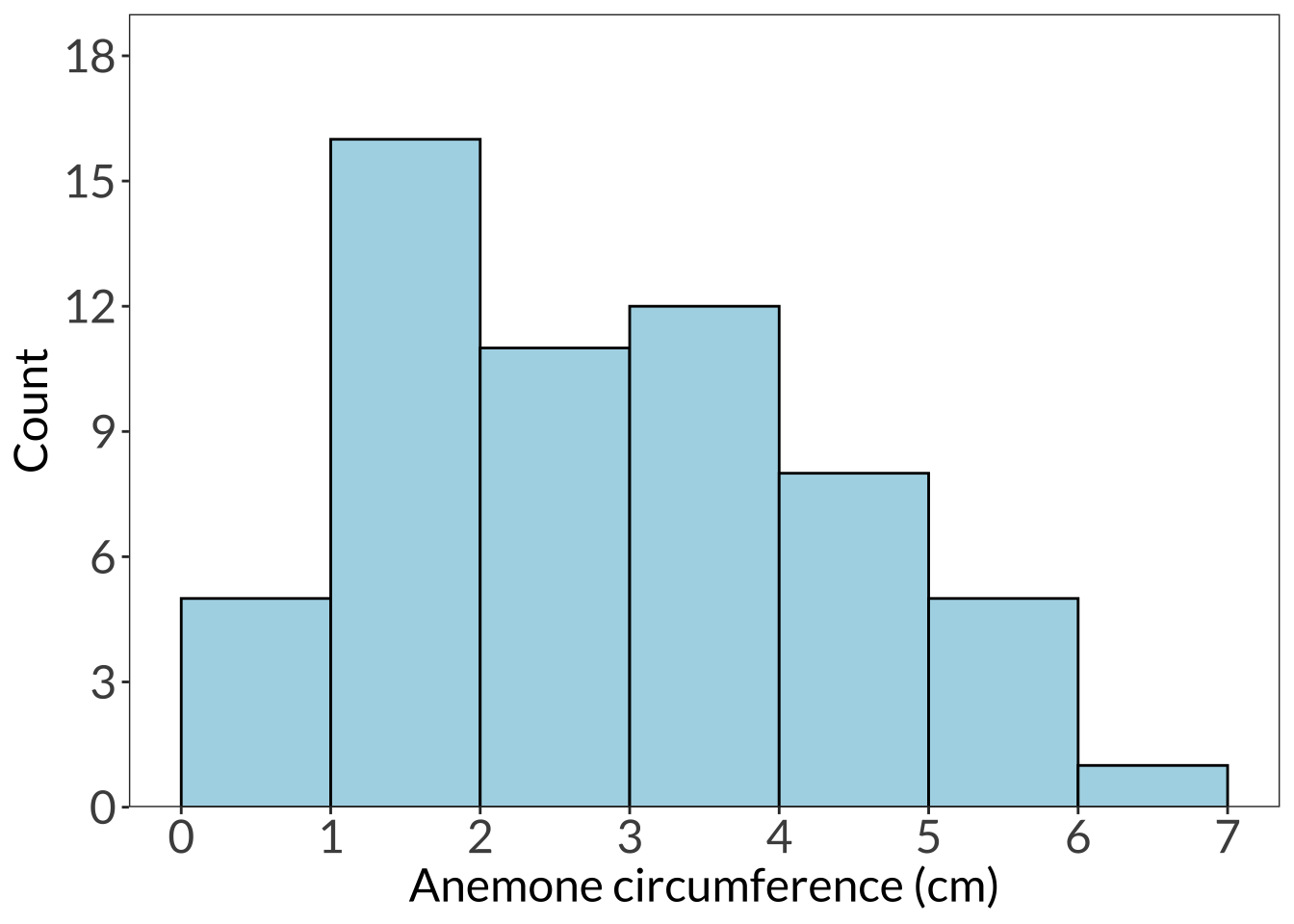

3. Probability mass example

Code

ggplot(data.frame(x = 1:55), aes(x)) +
  stat_function(geom = "bar", n = 55, fun = dpois, args = list(lambda = 10), fill = "coral") +
  scale_y_continuous(expand = c(0, 0), limits = c(0, 0.13)) +
  coord_cartesian(xlim = c(0, 22)) +
  labs(x = "Mussel clump size (count)", y = "Probability mass") +
  theme_bw() +
  theme(panel.grid = element_blank(),
        axis.text = element_text(size = 18),
        axis.title = element_text(size = 18),
        text = element_text(family = "Lato"))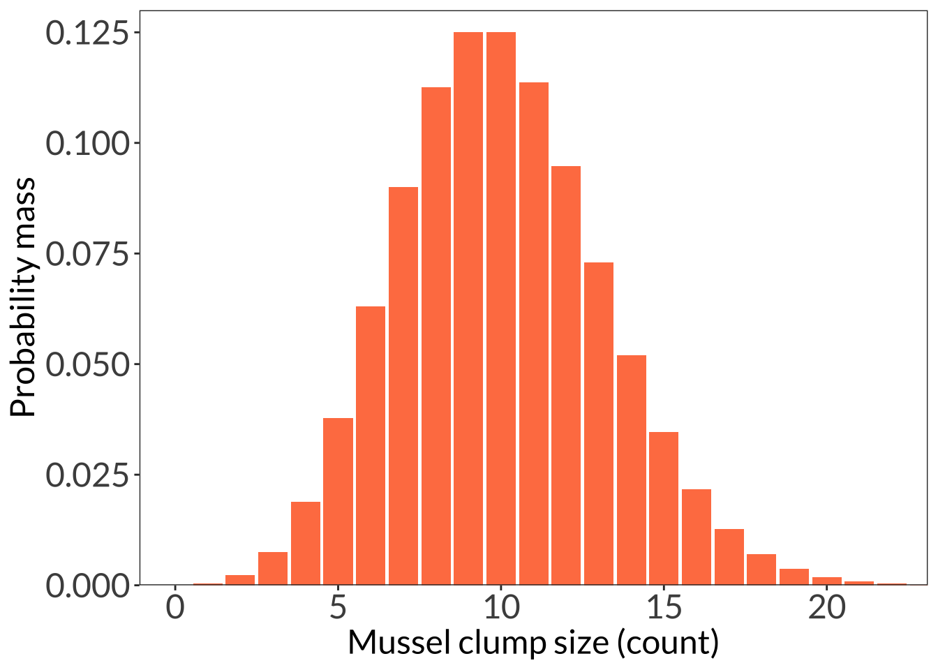

4. Probability density example

Code

ggplot(data.frame(x = 1:20), aes(x)) +
  stat_function(geom = "line", n = 100, fun = dnorm, args = list(mean = 10, sd = 2), linewidth = 1) +
  stat_function(geom = "area", fun = dnorm, args = list(mean = 10, sd = 2), xlim = c(12, 14), fill = "turquoise3") +
  geom_vline(xintercept = 12, lty = 2, color = "grey", linewidth = 1) +
  geom_vline(xintercept = 14, lty = 2, color = "grey", linewidth = 1) +
  scale_y_continuous(expand = c(0, 0), limits = c(0, 0.22)) +
  # coord_cartesian(xlim = c(0, 22)) +
  labs(x = "Individual mussel weight (g)", y = "Probability density") +
  theme_bw() +
  theme(panel.grid = element_blank(),
        axis.text = element_text(size = 18),
        axis.title = element_text(size = 18),
        text = element_text(family = "Lato"))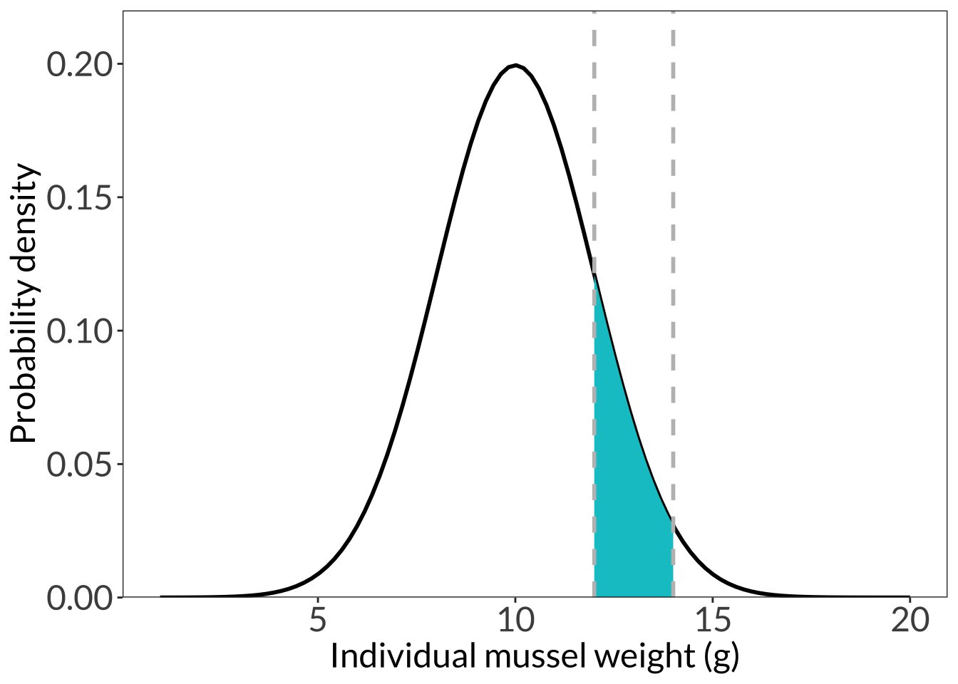

Code

showtext_auto(FALSE)

Citation

BibTeX citation:

@online{bui2023,
  author = {Bui, An},
  title = {Lecture 01 Figures},
  date = {2023-04-03},
  url = {https://an-bui.github.io/ES-193DS-W23/lecture/lecture-01_2023-04-03.html},
  langid = {en}
}

For attribution, please cite this work as:

Bui, An. 2023. “Lecture 01 Figures.” April 3, 2023. https://an-bui.github.io/ES-193DS-W23/lecture/lecture-01_2023-04-03.html.