0. set up

Code

# cleaning
library(tidyverse)

── Attaching core tidyverse packages ──────────────────────── tidyverse 2.0.0 ──
✔ dplyr     1.1.0     ✔ readr     2.1.4
✔ forcats   1.0.0     ✔ stringr   1.5.0
✔ ggplot2   3.4.1     ✔ tibble    3.2.0
✔ lubridate 1.9.2     ✔ tidyr     1.3.0
✔ purrr     1.0.1     
── Conflicts ────────────────────────────────────────── tidyverse_conflicts() ──
✖ dplyr::filter() masks stats::filter()
✖ dplyr::lag()    masks stats::lag()
ℹ Use the ]8;;http://conflicted.r-lib.org/conflicted package]8;; to force all conflicts to become errors

Code

# visualization
library(showtext)

Loading required package: sysfonts
Loading required package: showtextdb

Code

font_add_google("Lato", "Lato")
showtext_auto()

# panels together
library(patchwork)

# cohen's d
library(effsize)

1. one vs two tailed figure

Code

two <- ggplot(data.frame(x = -5:5), aes(x)) +
  stat_function(geom = "area", fun = dt, args = list(df = 1), xlim = c(3, 5), fill = "darkgrey") +
  geom_linerange(aes(x = 3, ymin = 0, ymax = 0.032), linewidth = 1, lty = 2, color = "#000000") +
  stat_function(geom = "area", fun = dt, args = list(df = 1), xlim = c(-5, -3), fill = "darkgrey") +
  geom_linerange(aes(x = -3, ymin = 0, ymax = 0.032), linewidth = 1, lty = 2, color = "#000000") +
  stat_function(geom = "line", n = 1000, fun = dt, args = list(df = 1), linewidth = 1, color = "#000000") +
  scale_y_continuous(expand = c(0, 0), limits = c(0, 0.32)) +
  theme_void() +
  theme(panel.grid = element_blank())

one <- ggplot(data.frame(x = -5:5), aes(x)) +
  stat_function(geom = "area", fun = dt, args = list(df = 1), xlim = c(2, 5), fill = "darkgrey") +
  geom_linerange(aes(x = 2, ymin = 0, ymax = 0.063), linewidth = 1, lty = 2, color = "#000000") +
  stat_function(geom = "line", n = 1000, fun = dt, args = list(df = 1), linewidth = 1, color = "#000000") +
  scale_y_continuous(expand = c(0, 0), limits = c(0, 0.32)) +
  theme_void() +
  theme(panel.grid = element_blank())

one + two

1. Acorn example

\[ \begin{align} n &= 41 \\ \bar{x} &= 2.29 \\ s &= 1.04 \end{align} \]

random numbers from t-distribution

Code

set.seed(7)
# acorns <- rt(n = 41, df = 40, ncp = 2.5) 
acorns <- rnorm(n = 41, mean = 2, sd = 1)

histogram

Code

hist <- enframe(acorns) %>% 
  ggplot(aes(x = value)) +
  geom_histogram(bins = 7, fill = "cornflowerblue", color = "#000000") +
  scale_y_continuous(expand = c(0, 0), limits = c(0, 11.5), breaks = c(0, 3, 6, 9, 12)) +
  theme_classic() +
  labs(x = "Acorn mass (g)", y = "Count")

qq plot

Code

qq <- enframe(acorns) %>% 
  ggplot(aes(sample = value)) +
  stat_qq_line(aes(sample = value)) +
  stat_qq(aes(sample = value), color = "cornflowerblue", size = 3) +
  theme_classic() +
  labs(x = "Theoretical quantiles", y = "Sample quantiles")

Code

hist + qq

calculating a critical value

Code

qt(p = .05/2, df = 40)

[1] -2.021075

calculating t-score

Code

# population mean
mu0 <- 2

# number of observations
n <- 41

# sample mean
xbar <- mean(acorns)

# sample standard deviation
s <- sd(acorns)

# sample standard error
se <- s/sqrt(n)

# degrees of freedom
df <- n - 1

# t-score
t <- (xbar-mu0)/se

t

[1] 1.803471

\[ t_s = \frac{\bar{x} - \mu}{s/\sqrt{n}} = \frac{2.29 - 2}{1.04/\sqrt{41}} = 1.8 \] ## visual representation of sample t-statistic vs t-critical

Code

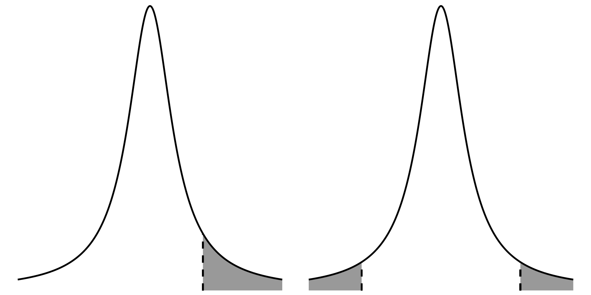
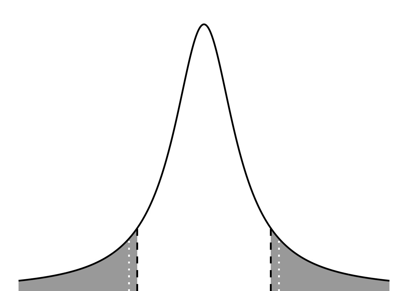
ggplot(data.frame(x = -5:5), aes(x)) +
  stat_function(geom = "area", fun = dt, args = list(df = 1), xlim = c(1.8, 5), fill = "darkgrey") +
  stat_function(geom = "area", fun = dt, args = list(df = 1), xlim = c(-5, -1.8), fill = "darkgrey") +
  geom_linerange(aes(x = 1.8, ymin = 0, ymax = 0.075), linewidth = 1, lty = 2, color = "#000000") +
  geom_linerange(aes(x = -1.8, ymin = 0, ymax = 0.075), linewidth = 1, lty = 2, color = "#000000") +
  
  geom_linerange(aes(x = 2.021, ymin = 0, ymax = 0.075), linewidth = 1, lty = 3, color = "#FFFFFF") +
  geom_linerange(aes(x = -2.021, ymin = 0, ymax = 0.075), linewidth = 1, lty = 3, color = "#FFFFFF") +
  stat_function(geom = "line", n = 1000, fun = dt, args = list(df = 1), linewidth = 1, color = "#000000") +
  scale_y_continuous(expand = c(0, 0), limits = c(0, 0.32)) +
  theme_void() +
  theme(panel.grid = element_blank(),
        plot.margin = unit(c(1, 0, 0, 0), "cm"))

manually calculating p-value

Code

# two-tailed: multiply probability by 2
# lower = FALSE: probability of the value being more than t
2*pt(t, df, lower = FALSE)

[1] 0.07885024

doing a t-test

Code

t.test(acorns, mu = 2)


    One Sample t-test

data:  acorns
t = 1.8035, df = 40, p-value = 0.07885
alternative hypothesis: true mean is not equal to 2
95 percent confidence interval:
 1.964535 2.623323
sample estimates:
mean of x 
 2.293929

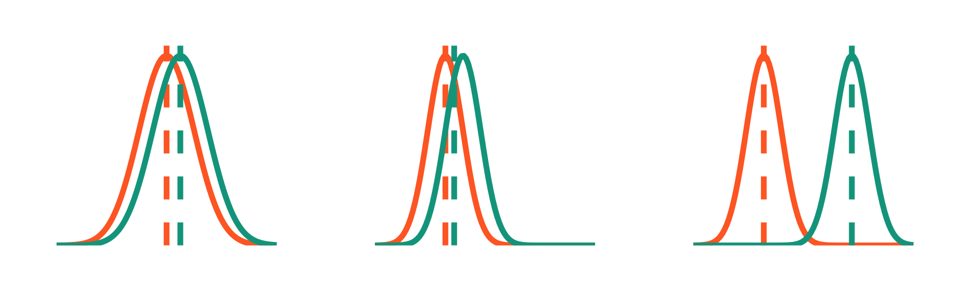
2. two-sample t-test

Code

ex1 <- ggplot(data.frame(x = -8:8), aes(x)) +
  stat_function(geom = "line", n = 100, fun = dnorm, args = list(mean = 0, sd = 2), linewidth = 2, color = "#FF6B2B") +
  geom_vline(aes(xintercept = 0), color = "#FF6B2B", lty = 2, linewidth = 2) +
  stat_function(geom = "line", n = 100, fun = dnorm, args = list(mean = 1, sd = 2), linewidth = 2, color = "#00A38D") +
  geom_vline(aes(xintercept = 1), color = "#00A38D", lty = 2, linewidth = 2) +
    scale_y_continuous(expand = c(0, 0), limits = c(0, 0.21)) +
  theme_void() +
  theme(plot.margin = unit(c(1, 1, 1, 1), "cm"))

set.seed(2)
x <- rnorm(30, mean = 0, sd = 2)
y <- rnorm(30, mean = 1, sd = 2)

t.test(x = x, y = y, var.equal = TRUE)


    Two Sample t-test

data:  x and y
t = -0.78852, df = 58, p-value = 0.4336
alternative hypothesis: true difference in means is not equal to 0
95 percent confidence interval:
 -1.6721807  0.7270662
sample estimates:
mean of x mean of y 
0.4573436 0.9299009

Code

# 0.43

Code

ex2 <- ggplot(data.frame(x = -8:17), aes(x)) +
  stat_function(geom = "line", n = 100, fun = dnorm, args = list(mean = 0, sd = 2), linewidth = 2, color = "#FF6B2B") +
  geom_vline(aes(xintercept = 0), color = "#FF6B2B", lty = 2, linewidth = 2) +
  stat_function(geom = "line", n = 100, fun = dnorm, args = list(mean = 2, sd = 2), linewidth = 2, color = "#00A38D") +
  geom_vline(aes(xintercept = 1), color = "#00A38D", lty = 2, linewidth = 2) +
    scale_y_continuous(expand = c(0, 0), limits = c(0, 0.21)) +
  theme_void() +
  theme(plot.margin = unit(c(1, 1, 1, 1), "cm"))

set.seed(1000000000)
x <- rnorm(30, mean = 0, sd = 2)
y <- rnorm(30, mean = 2, sd = 2)

t.test(x = x, y = y, var.equal = TRUE)


    Two Sample t-test

data:  x and y
t = -3.7904, df = 58, p-value = 0.0003603
alternative hypothesis: true difference in means is not equal to 0
95 percent confidence interval:
 -2.7905631 -0.8617609
sample estimates:
mean of x mean of y 
0.1435745 1.9697364

Code

# 0.6932

Code

ex3 <- ggplot(data.frame(x = -8:17), aes(x)) +
  stat_function(geom = "line", n = 100, fun = dnorm, args = list(mean = 0, sd = 2), linewidth = 2, color = "#FF6B2B") +
  geom_vline(aes(xintercept = 0), color = "#FF6B2B", lty = 2, linewidth = 2) +
  stat_function(geom = "line", n = 100, fun = dnorm, args = list(mean = 10, sd = 2), linewidth = 2, color = "#00A38D") +
  geom_vline(aes(xintercept = 10), color = "#00A38D", lty = 2, linewidth = 2) +
    scale_y_continuous(expand = c(0, 0), limits = c(0, 0.21)) +
  theme_void() +
  theme(plot.margin = unit(c(1, 1, 1, 1), "cm"))

set.seed(100)
x <- rnorm(40, mean = 0, sd = 2)
y <- rnorm(40, mean = 10, sd = 2)

t.test(x = x, y = y, var.equal = TRUE)


    Two Sample t-test

data:  x and y
t = -21.69, df = 78, p-value < 2.2e-16
alternative hypothesis: true difference in means is not equal to 0
95 percent confidence interval:
 -10.564878  -8.788488
sample estimates:
mean of x mean of y 
0.2003543 9.8770375

Code

# p < 0.001

Code

ex1 + ex2 + ex3

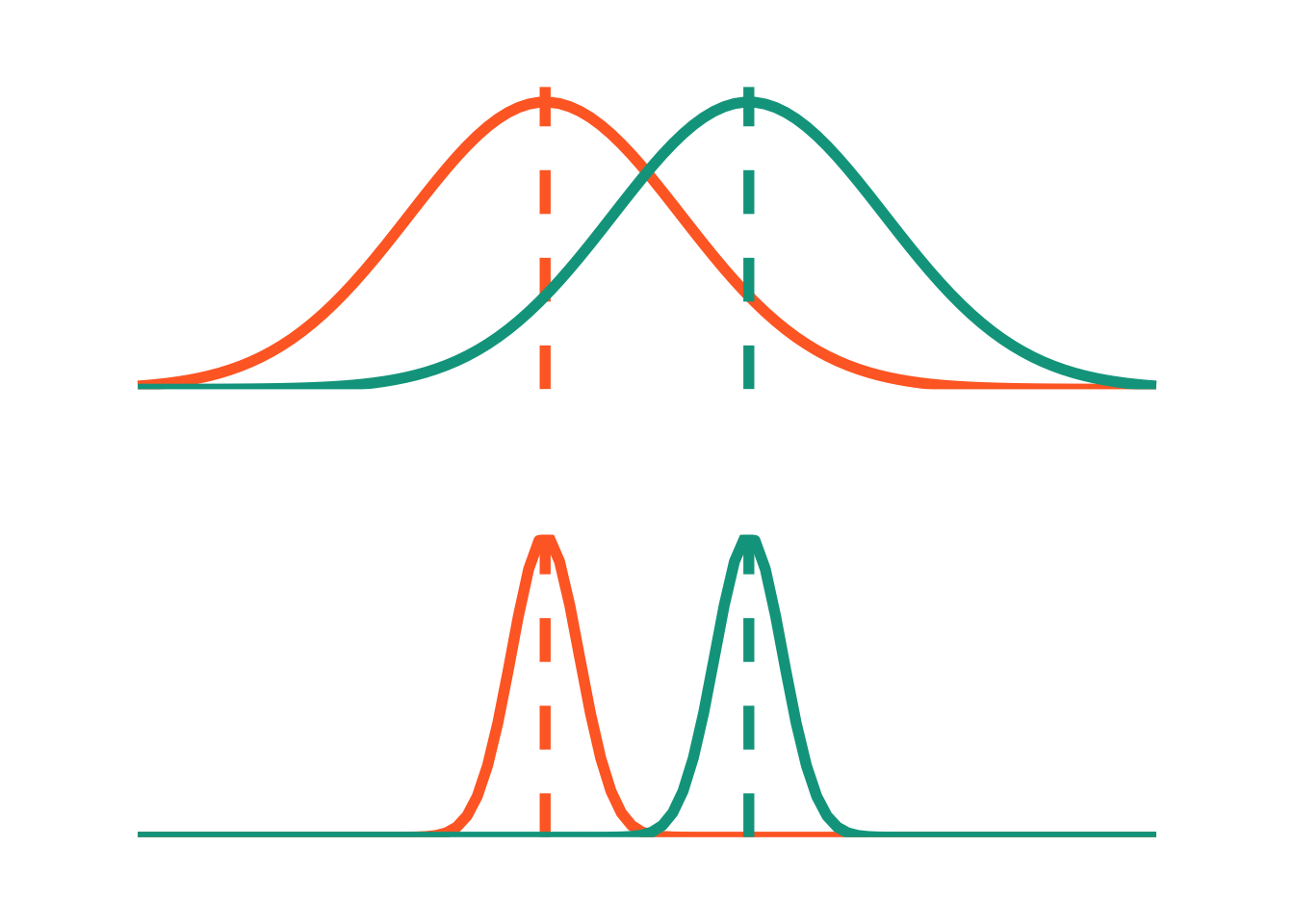
same differences in means, different SD

Code

small <- ggplot(data.frame(x = -6:9), aes(x)) +
  stat_function(geom = "line", n = 100, fun = dnorm, args = list(mean = 0, sd = 2), linewidth = 2, color = "#FF6B2B") +
  geom_vline(aes(xintercept = 0), color = "#FF6B2B", lty = 2, linewidth = 2) +
  stat_function(geom = "line", n = 100, fun = dnorm, args = list(mean = 3, sd = 2), linewidth = 2, color = "#00A38D") +
  geom_vline(aes(xintercept = 3), color = "#00A38D", lty = 2, linewidth = 2) +
    scale_y_continuous(expand = c(0, 0), limits = c(0, 0.21)) +
  theme_void() +
  theme(plot.margin = unit(c(1, 1, 1, 1), "cm"))

big <- ggplot(data.frame(x = -6:9), aes(x)) +
  stat_function(geom = "line", n = 100, fun = dnorm, args = list(mean = 0, sd = 0.5), linewidth = 2, color = "#FF6B2B") +
  geom_vline(aes(xintercept = 0), color = "#FF6B2B", lty = 2, linewidth = 2) +
  stat_function(geom = "line", n = 100, fun = dnorm, args = list(mean = 3, sd = 0.5), linewidth = 2, color = "#00A38D") +
  geom_vline(aes(xintercept = 3), color = "#00A38D", lty = 2, linewidth = 2) +
    scale_y_continuous(expand = c(0, 0), limits = c(0, 0.8)) +
  theme_void() +
  theme(plot.margin = unit(c(1, 1, 1, 1), "cm"))

small / big

3. Cohen’s D

\[ Cohen's d = \frac{\bar{x_A} - \bar{x_B}}{\sqrt{(s^2_A + s^2_B)/2}} \]

Code

cohen.d(acorns ~ ., mu = 2)


Cohen's d (single sample)

d estimate: 0.2816548 (small)
Reference mu: 2
95 percent confidence interval:
     lower      upper 
-0.3527453  0.9160549

Citation

BibTeX citation:

@online{bui2023,
  author = {Bui, An},
  title = {Lecture 04 Figures},
  date = {2023-04-24},
  url = {https://an-bui.github.io/ES-193DS-W23/lecture/lecture-04_2023-04-24.html},
  langid = {en}
}

For attribution, please cite this work as:

Bui, An. 2023. “Lecture 04 Figures.” April 24, 2023. https://an-bui.github.io/ES-193DS-W23/lecture/lecture-04_2023-04-24.html.