Code

library(tidyverse)
library(palmerpenguins)
library(showtext)
library(car)
font_add_google("Lato", "Lato")
showtext_auto()
library(patchwork)

Chi-square

test statistic:

\[ \chi^2 = \Sigma\frac{(O-E)^2}{E} \] ### degrees of freedom \[ df = (number\;of\;rows - 1) * (number\;of\;columns - 1) \]

expected counts:

\[ expected = \frac{row\;total * column\;total}{table\;total} \]

expected counts example from lecture

\[ \frac{126 * 118}{315} = 47.2 \]

test statistic calculation example from lecture

\[ \begin{align} \chi^2 &= \Sigma\frac{(O-E)^2}{E} \\ \chi^2 &= \frac{55-47.2}{47.2}+...+\frac{45-31.9}{31.9} \\ &= 15.276 \end{align} \]

example code

Code

# create matrix
survey <- tribble(
  ~distance, ~trails, ~dog_access, ~wildlife_habitat,
  "walking_distance", 55, 38, 33,
  "driving_distance", 41, 25, 29,
  "out_of_town", 22, 27, 45
) %>% 
  column_to_rownames("distance")

survey

                 trails dog_access wildlife_habitat
walking_distance     55         38               33
driving_distance     41         25               29
out_of_town          22         27               45

Code

# calculate proportions
survey_summary <- tribble(
  ~distance, ~trails, ~dog_access, ~wildlife_habitat,
  "walking_distance", 55, 38, 33,
  "driving_distance", 41, 25, 29,
  "out_of_town", 22, 27, 45
) %>% 
  pivot_longer(cols = trails:wildlife_habitat, names_to = "responses", values_to = "counts") %>% 
  group_by(distance) %>% 
  mutate(sum = sum(counts)) %>% 
  ungroup() %>% 
  mutate(prop = counts/sum)
  
# do chi-square
chisq.test(survey)


    Pearson's Chi-squared test

data:  survey
X-squared = 15.276, df = 4, p-value = 0.004162

Code

# get expected matrix
chisq.test(survey)$expected

                  trails dog_access wildlife_habitat
walking_distance 47.2000   36.00000         42.80000
driving_distance 35.5873   27.14286         32.26984
out_of_town      35.2127   26.85714         31.93016

ANOVA

ANOVA variance figure:

Code

col1 <- "cornflowerblue"
col2 <- "orange"
col3 <- "darkgreen"

ggplot(data.frame(x = 0:22), aes(x)) +
  stat_function(geom = "line", n = 100, fun = dnorm, args = list(mean = 10, sd = 2), linewidth = 1, col = col1) + 
  stat_function(geom = "line", n = 100, fun = dnorm, args = list(mean = 8, sd = 2), linewidth = 1, col = col2) +
  stat_function(geom = "line", n = 100, fun = dnorm, args = list(mean = 15, sd = 2), linewidth = 1, col = col3) +
  theme_bw() +
  theme(panel.grid = element_blank(),
        axis.text = element_blank(),
        axis.title = element_blank(),
        axis.ticks = element_blank(),
        panel.border = element_blank(),
        text = element_text(family = "Lato"))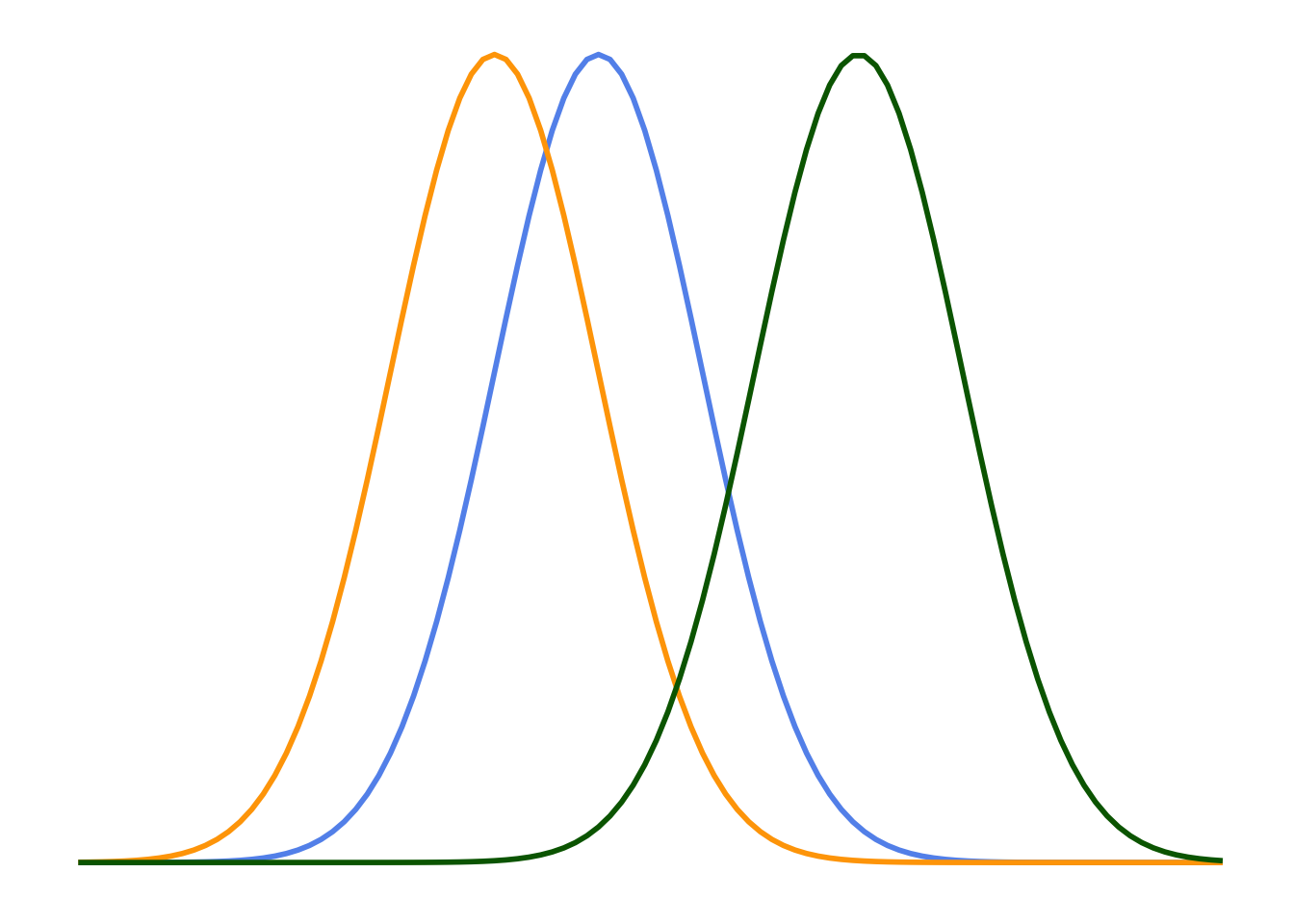

ANOVA with palmer penguins

Code

# Adelie: 10
# Chinstrap: 8
# Gentoo: 10

adelie <- penguins %>% 
  filter(species == "Adelie")

adelie_hist <- ggplot(data = adelie, aes(x = bill_length_mm)) +
  geom_histogram(bins = 10, fill = col1, color = col1, alpha = 0.8) +
  labs(x = "Bill length (mm)", y = "Count") +
  theme_bw() +
  theme(panel.grid = element_blank(),
        axis.text = element_text(size = 18),
        axis.title = element_text(size = 18),
        axis.ticks = element_blank(),
        text = element_text(family = "Lato")) 

adelie_qq <- ggplot(data = adelie, aes(sample = bill_length_mm)) +
  stat_qq_line(linewidth = 1) +
  stat_qq(col = col1) +
  labs(x = "Theoretical", y = "Sample") +
  theme_bw() +
  theme(panel.grid = element_blank(),
        axis.text = element_text(size = 18),
        axis.title = element_text(size = 18),
        axis.ticks = element_blank(),
        text = element_text(family = "Lato")) 

shapiro.test(adelie$bill_length_mm)


    Shapiro-Wilk normality test

data:  adelie$bill_length_mm
W = 0.99336, p-value = 0.7166

Code

chinstrap <- penguins %>% 
  filter(species == "Chinstrap")

chinstrap_hist <- ggplot(data = chinstrap, aes(x = bill_length_mm)) +
  geom_histogram(bins = 10, fill = col2, color = col2, alpha = 0.8) +
  labs(x = "Bill length (mm)", y = "Count") +
  theme_bw() +
  theme(panel.grid = element_blank(),
        axis.text = element_text(size = 18),
        axis.title = element_text(size = 18),
        axis.ticks = element_blank(),
        text = element_text(family = "Lato")) 

chinstrap_qq <- ggplot(data = chinstrap, aes(sample = bill_length_mm)) +
  stat_qq_line(linewidth = 1) +
  stat_qq(col = col2) +
  labs(x = "Theoretical", y = "Sample") +
  theme_bw() +
  theme(panel.grid = element_blank(),
        axis.text = element_text(size = 18),
        axis.title = element_text(size = 18),
        axis.ticks = element_blank(),
        text = element_text(family = "Lato")) 

shapiro.test(chinstrap$bill_length_mm)


    Shapiro-Wilk normality test

data:  chinstrap$bill_length_mm
W = 0.97525, p-value = 0.1941

Code

gentoo <- penguins %>% 
  filter(species == "Gentoo")

gentoo_hist <- ggplot(data = gentoo, aes(x = bill_length_mm)) +
  geom_histogram(bins = 10, fill = col3, color = col3, alpha = 0.8) +
  labs(x = "Bill length (mm)", y = "Count") +
  theme_bw() +
  theme(panel.grid = element_blank(),
        axis.text = element_text(size = 18),
        axis.title = element_text(size = 18),
        axis.ticks = element_blank(),
        text = element_text(family = "Lato")) 

gentoo_qq <- ggplot(data = gentoo, aes(sample = bill_length_mm)) +
  stat_qq_line(linewidth = 1) +
  stat_qq(col = col3) +
  labs(x = "Theoretical", y = "Sample") +
  theme_bw() +
  theme(panel.grid = element_blank(),
        axis.text = element_text(size = 18),
        axis.title = element_text(size = 18),
        axis.ticks = element_blank(),
        text = element_text(family = "Lato")) 


(adelie_hist + adelie_qq) / (chinstrap_hist + chinstrap_qq) / (gentoo_hist + gentoo_qq)

Warning: Removed 1 rows containing non-finite values (`stat_bin()`).

Warning: Removed 1 rows containing non-finite values (`stat_qq_line()`).

Warning: Removed 1 rows containing non-finite values (`stat_qq()`).

Warning: Removed 1 rows containing non-finite values (`stat_bin()`).

Warning: Removed 1 rows containing non-finite values (`stat_qq_line()`).

Warning: Removed 1 rows containing non-finite values (`stat_qq()`).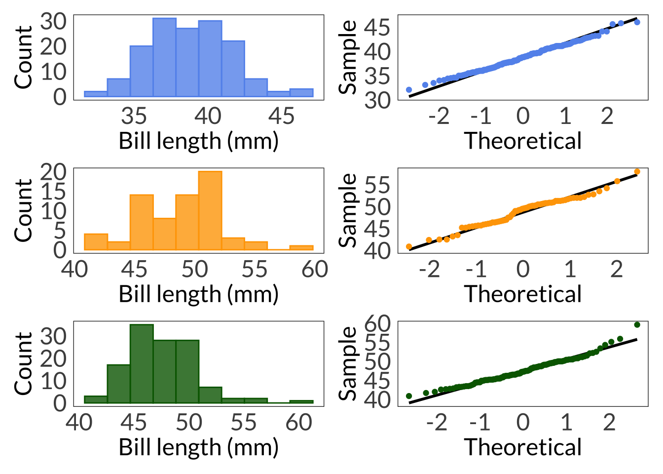

Code

shapiro.test(gentoo$bill_length_mm)


    Shapiro-Wilk normality test

data:  gentoo$bill_length_mm
W = 0.97272, p-value = 0.01349

Code

leveneTest(bill_length_mm ~ species, data = penguins)

Levene's Test for Homogeneity of Variance (center = median)
       Df F value Pr(>F)
group   2  2.2425 0.1078
      339

Code

penguins_anova <- aov(bill_length_mm ~ species, data = penguins)
penguins_anova

Call:
   aov(formula = bill_length_mm ~ species, data = penguins)

Terms:
                 species Residuals
Sum of Squares  7194.317  2969.888
Deg. of Freedom        2       339

Residual standard error: 2.959853
Estimated effects may be unbalanced
2 observations deleted due to missingness

Code

summary(penguins_anova)

             Df Sum Sq Mean Sq F value Pr(>F)    
species       2   7194    3597   410.6 <2e-16 ***
Residuals   339   2970       9                   
---
Signif. codes:  0 '***' 0.001 '**' 0.01 '*' 0.05 '.' 0.1 ' ' 1
2 observations deleted due to missingness

Code

TukeyHSD(penguins_anova)

  Tukey multiple comparisons of means
    95% family-wise confidence level

Fit: aov(formula = bill_length_mm ~ species, data = penguins)

$species
                      diff       lwr        upr     p adj
Chinstrap-Adelie 10.042433  9.024859 11.0600064 0.0000000
Gentoo-Adelie     8.713487  7.867194  9.5597807 0.0000000
Gentoo-Chinstrap -1.328945 -2.381868 -0.2760231 0.0088993

ANOVA information

Sum of squares

among groups

\[ \sum_{i=1}^{k}\sum_{j=1}^{n}(\bar{x}_i - \bar{x})^2 \]

within groups

\[ \sum_{i=1}^{k}\sum_{j=1}^{n}({x}_{ij} - \bar{x}_i)^2 \]

total

\[ \sum_{i=1}^{k}\sum_{j=1}^{n}({x}_{ij} - \bar{x})^2 \]

Mean squares

among groups

\[ \frac{SS_{among\;group}}{k-1} \] #### within group

\[ \frac{SS_{within\;group}}{n-k} \] #### total

\[ \frac{SS_{total}}{kn-1} \]

F-ratio

\[ \frac{MS_{among\;group}}{MS_{within\;group}} \]

penguins visualization

Code

ggplot(data = penguins, aes(x = species, y = bill_length_mm, fill = species)) +
  geom_violin(alpha = 0.6) +
  geom_boxplot(width = 0.2) +
  scale_fill_manual(values = c(col1, col2, col3)) +
  labs(x = "Species", y = "Bill length (mm)") +
  theme_bw() +
  theme(panel.grid = element_blank(),
        axis.text = element_text(size = 18),
        axis.title = element_text(size = 18),
        text = element_text(family = "Lato"),
        legend.position = "none")

Warning: Removed 2 rows containing non-finite values (`stat_ydensity()`).

Warning: Removed 2 rows containing non-finite values (`stat_boxplot()`).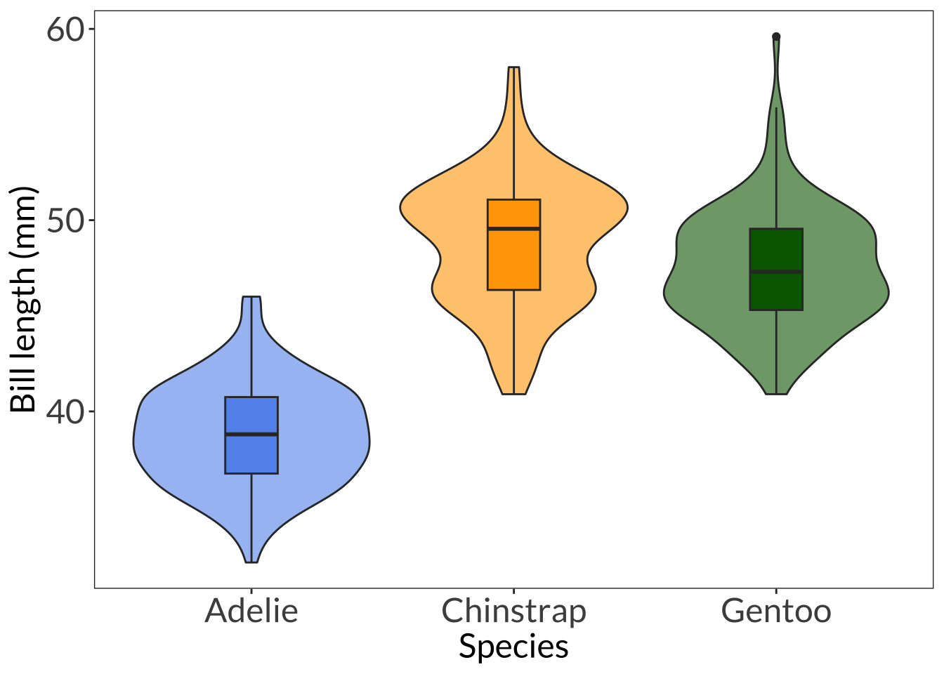

Kruskal-Wallis

test statistic

\[ H = \frac{12}{n(n+1)}\sum_{i = 1}^{k}\frac{R^2_i}{n_i}-3(n+1) \]

eta squared

\[ \eta^2 = \frac{H - k + 1}{n - k} \]

Citation

BibTeX citation:

@online{bui2023,
  author = {Bui, An},
  title = {Lecture 06 Figures},
  date = {2023-05-08},
  url = {https://an-bui.github.io/ES-193DS-W23/lecture/lecture-06_2023-05-08.html},
  langid = {en}
}

For attribution, please cite this work as:

Bui, An. 2023. “Lecture 06 Figures.” May 8, 2023. https://an-bui.github.io/ES-193DS-W23/lecture/lecture-06_2023-05-08.html.