Code

library(tidyverse)
library(palmerpenguins)
library(showtext)
library(car)
font_add_google("Lato", "Lato")
showtext_auto()
library(patchwork)
library(ggeffects)
library(performance)
library(broom)
library(flextable)

what is a residual?

\[ residual = y_i - \hat{y} \]

\[ SS_{residuals} = (-1)^2 + (4)^2 + (-2)^2 + (-3)^2 = 30 \] # R2

\[ \begin{align} R^2 &= 1 - \frac{\sum_{i = 1}^{n}(y_i - \hat{y})^2}{\sum_{i = 1}^{n}(y_i - \bar{y})^2} \\ &= 1 - \frac{SS_{residuals}}{SS_{total}} \end{align} \]

linear model equation

\[ \begin{align} y &= mx + b \\ y &= b_1x + b_0 + \epsilon = b_0 + b_1x + \epsilon \\ y &= \beta_1x + \beta_0 + \epsilon = \beta_0 + \beta_1x + \epsilon \end{align} \]

linear model hypotheses

\[ \begin{align} H_0 &: \beta_1 = 0 \\ H_A &: \beta_1 \not = 0 \end{align} \]

what are we doing when we fit a linear model?

Code

set.seed(666)
data <- cbind(x = 1:5, y = rnorm(5, mean = 2, sd = 1)*1:5) %>% 
  as.data.frame()

noline <- ggplot(data, aes(x = x, y = y)) +
  geom_point(size = 5, color = "darkgreen", fill = "slategrey", shape = 21, stroke = 3) +
  theme_classic() +
  labs(x = "Predictor", y = "Response") +
  theme(text = element_text(size = 14))

opt1 <- ggplot(data, aes(x = x, y = y)) +
  geom_point(size = 5, color = "darkgreen", fill = "slategrey", shape = 21, stroke = 3) +
  geom_function(fun = function(x) 2*x, color = "coral2", linewidth = 2, lty = 2) +
  theme_classic() +
  labs(x = "Predictor", y = "Response") +
  theme(text = element_text(size = 14))

opt2 <- ggplot(data, aes(x = x, y = y)) +
  geom_point(size = 5, color = "darkgreen", fill = "slategrey", shape = 21, stroke = 3) +
  geom_function(fun = function(x) -2*x + 10, color = "coral2", linewidth = 2, lty = 2) +
  theme_classic() +
  labs(x = "Predictor", y = "Response") +
  theme(text = element_text(size = 14))

Code

no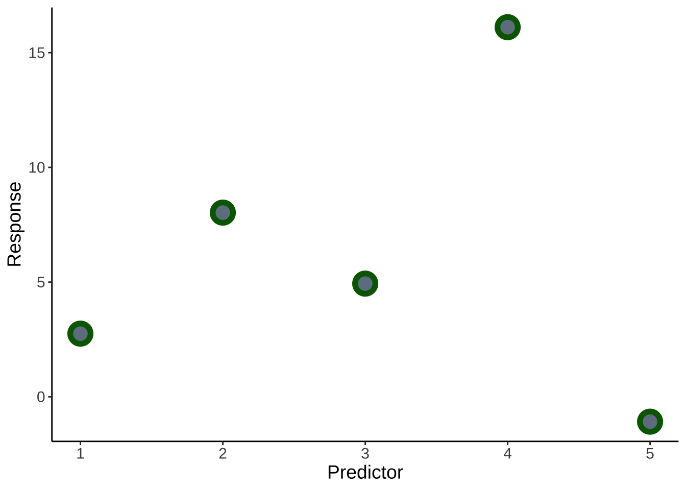line

Code

opt1 / opt2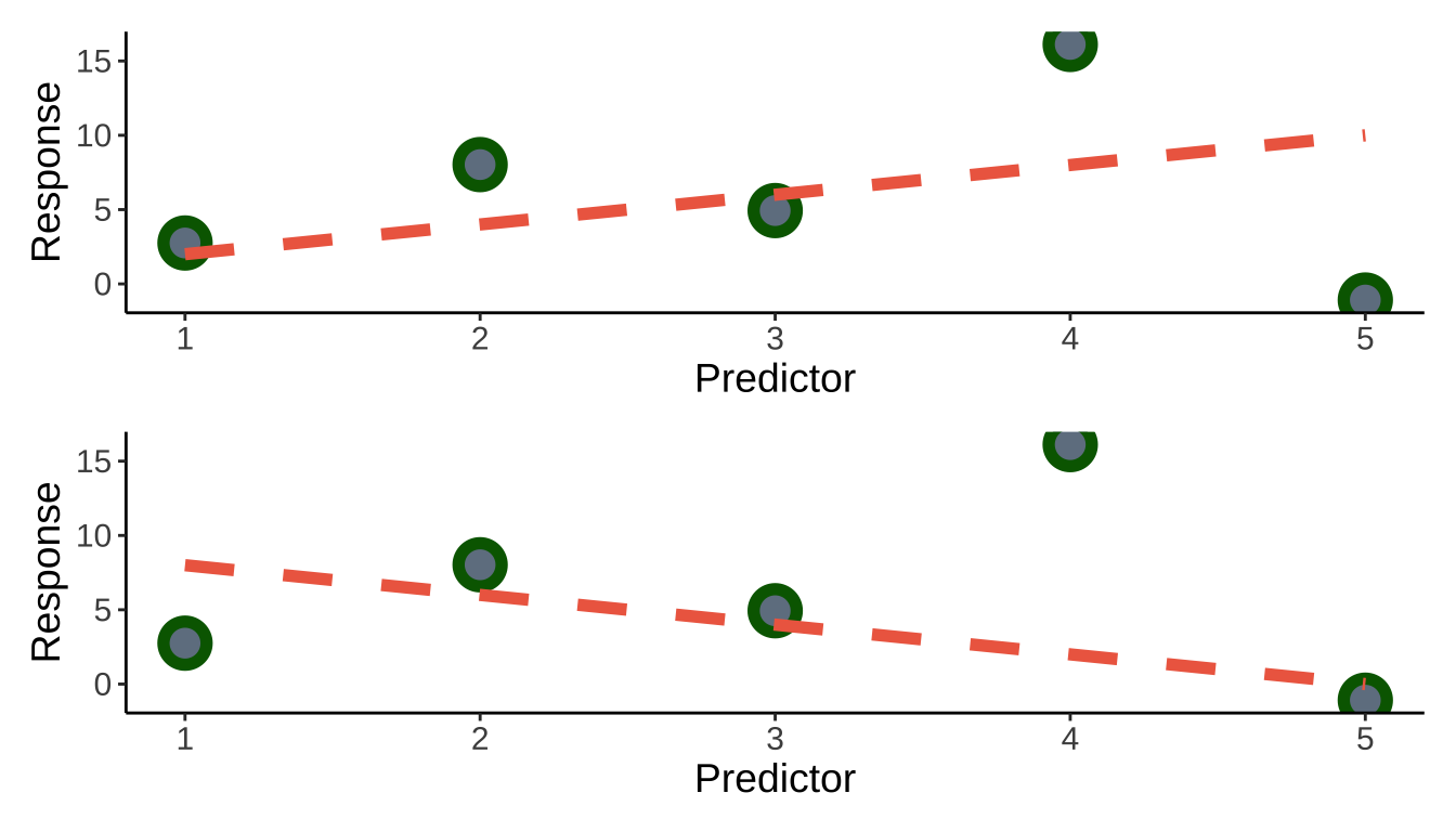

actual linear relationship example

generating data and model

Code

x_lm <- seq(from = 1, to = 30, by = 1)

set.seed(666)
y_lm <- round(runif(length(x_lm), min = 1, max = 1.5), 1)*x_lm + runif(length(x_lm), min = 1, max = 10)

df_lm <- cbind(
  x = x_lm,
  y = y_lm
) %>% 
  as_tibble() %>% 
  mutate(outlier = case_when(
    rownames(.) %in% c(23, 27, 28) ~ "outlier",
    TRUE ~ "ok"
  ))

model summaries

Code

model1 <- lm(y ~ x, data = df_lm)
model1


Call:
lm(formula = y ~ x, data = df_lm)

Coefficients:
(Intercept)            x  
      6.404        1.156

Code

summary(model1)


Call:
lm(formula = y ~ x, data = df_lm)

Residuals:
   Min     1Q Median     3Q    Max 
-8.323 -1.020  0.002  2.393  6.645 

Coefficients:
            Estimate Std. Error t value Pr(>|t|)    
(Intercept)   6.4043     1.3421   4.772 5.17e-05 ***
x             1.1561     0.0756  15.293 4.02e-15 ***
---
Signif. codes:  0 '***' 0.001 '**' 0.01 '*' 0.05 '.' 0.1 ' ' 1

Residual standard error: 3.584 on 28 degrees of freedom
Multiple R-squared:  0.8931,    Adjusted R-squared:  0.8893 
F-statistic: 233.9 on 1 and 28 DF,  p-value: 4.021e-15

Code

anova(model1)

Analysis of Variance Table

Response: y
          Df  Sum Sq Mean Sq F value    Pr(>F)    
x          1 3003.92 3003.92  233.87 4.021e-15 ***
Residuals 28  359.64   12.84                      
---
Signif. codes:  0 '***' 0.001 '**' 0.01 '*' 0.05 '.' 0.1 ' ' 1

Code

model1_nooutliers <- lm(y ~ x, data = df_lm %>% filter(outlier == "ok"))
summary(model1_nooutliers)


Call:
lm(formula = y ~ x, data = df_lm %>% filter(outlier == "ok"))

Residuals:
    Min      1Q  Median      3Q     Max 
-6.6611 -1.2596 -0.5039  1.6229  4.7197 

Coefficients:
            Estimate Std. Error t value Pr(>|t|)    
(Intercept)  6.12314    1.02352   5.982 3.02e-06 ***
x            1.20027    0.06177  19.431  < 2e-16 ***
---
Signif. codes:  0 '***' 0.001 '**' 0.01 '*' 0.05 '.' 0.1 ' ' 1

Residual standard error: 2.668 on 25 degrees of freedom
Multiple R-squared:  0.9379,    Adjusted R-squared:  0.9354 
F-statistic: 377.6 on 1 and 25 DF,  p-value: < 2.2e-16

\[ \begin{align} R^2 &= 1 - \frac{SS_{residuals}}{SS_{total}} \\ &= 1 - \frac{359.64}{359.64 + 3003.92} \\ &= 0.8931 \end{align} \]

Code

# if using quarto, don't label chunk with a table... so weird
anova_tbl <- broom::tidy(anova(model1)) %>% 
  mutate(across(where(is.numeric), ~ round(.x, digits = 2))) %>% 
  mutate(p.value = case_when(
    p.value < 0.001 ~ "< 0.001"
  )) 

flextable(anova_tbl) %>% 
  set_header_labels(term = "Term", 
                    df = "Degrees of freedom", 
                    sumsq = "Sum of squares", 
                    meansq = "Mean squares", 
                    statistic = "F-statistic", 
                    p.value = "p-value") %>% 
  set_table_properties(layout = "autofit", width = 0.8)

Term	Degrees of freedom	Sum of squares	Mean squares	F-statistic	p-value
x	1	3,003.92	3,003.92	233.87	< 0.001
Residuals	28	359.64	12.84

model plots

Code

model1_pred <- ggpredict(model1, terms = ~ x)
model1_nooutliers_pred <- ggpredict(model1_nooutliers, terms = ~ x)

model1_plot_noline <- ggplot(data = df_lm, aes(x = x, y = y)) +
  geom_point(shape = 19, size = 3, color = "cornflowerblue") +
  theme_classic() +
  theme(text = element_text(size = 14))

model1_plot <- ggplot(data = df_lm, aes(x = x, y = y)) +
  geom_point(shape = 19, size = 3, color = "cornflowerblue") +
  geom_line(data = model1_pred, aes(x = x, y = predicted), linewidth = 1) +
  theme_classic() +
  theme(text = element_text(size = 14))

model1_plot_nooutliers <- ggplot(data = df_lm %>% filter(outlier == "ok"), aes(x = x, y = y)) +
  geom_point(aes(color = outlier), shape = 19, size = 3) +
  scale_color_manual(values = c("ok" = "cornflowerblue", "outlier" = "red")) +
  geom_line(data = model1_nooutliers_pred, aes(x = x, y = predicted), linewidth = 1) +
  theme_classic() +
  theme(text = element_text(size = 14),
        legend.position = "none")

exponential growth example

Code

x_ex <- seq(from = 5, to = 9, length = 30)

y_ex <- exp(x_ex)

df_ex <- cbind(
  x = x_ex,
  y = exp(x_ex)
) %>% 
  as_tibble()

lm_ex <- lm(y ~ x, data = df_ex)

lm_ex


Call:
lm(formula = y ~ x, data = df_ex)

Coefficients:
(Intercept)            x  
      -9431         1642

model summary

Code

summary(lm_ex)


Call:
lm(formula = y ~ x, data = df_ex)

Residuals:
    Min      1Q  Median      3Q     Max 
-1081.0  -843.2  -226.3   660.5  2756.1 

Coefficients:
            Estimate Std. Error t value Pr(>|t|)    
(Intercept)  -9431.3     1111.3  -8.486 3.16e-09 ***
x             1642.0      156.5  10.492 3.30e-11 ***
---
Signif. codes:  0 '***' 0.001 '**' 0.01 '*' 0.05 '.' 0.1 ' ' 1

Residual standard error: 1023 on 28 degrees of freedom
Multiple R-squared:  0.7972,    Adjusted R-squared:   0.79 
F-statistic: 110.1 on 1 and 28 DF,  p-value: 3.298e-11

model plots

Code

lm_pred <- ggpredict(lm_ex, terms = ~x)

ex_plot_noline <- ggplot(df_ex, aes(x= x, y = y)) +
  geom_point(shape = 17, size = 3, color = "orange") +
  theme_classic() +
  theme(text = element_text(size = 14))

ex_plot <- ggplot(df_ex, aes(x= x, y = y)) +
  geom_point(shape = 17, size = 3, color = "orange") +
  geom_line(data = lm_pred, aes(x = x, y = predicted), linewidth = 1) +
  theme_classic() +
  theme(text = element_text(size = 14))

diagnostic plots

Code

par(mfrow = c(2, 4))
plot(model1, which = c(1), col = "cornflowerblue", pch = 19)
plot(lm_ex, which = c(1), col = "orange", pch = 17)
plot(model1, which = c(2), col = "cornflowerblue", pch = 19)
plot(lm_ex, which = c(2), col = "orange", pch = 17)
plot(model1, which = c(3), col = "cornflowerblue", pch = 19)
plot(lm_ex, which = c(3), col = "orange", pch = 17)
plot(model1, which = c(5), col = "cornflowerblue", pch = 19)
plot(lm_ex, which = c(5), col = "orange", pch = 17)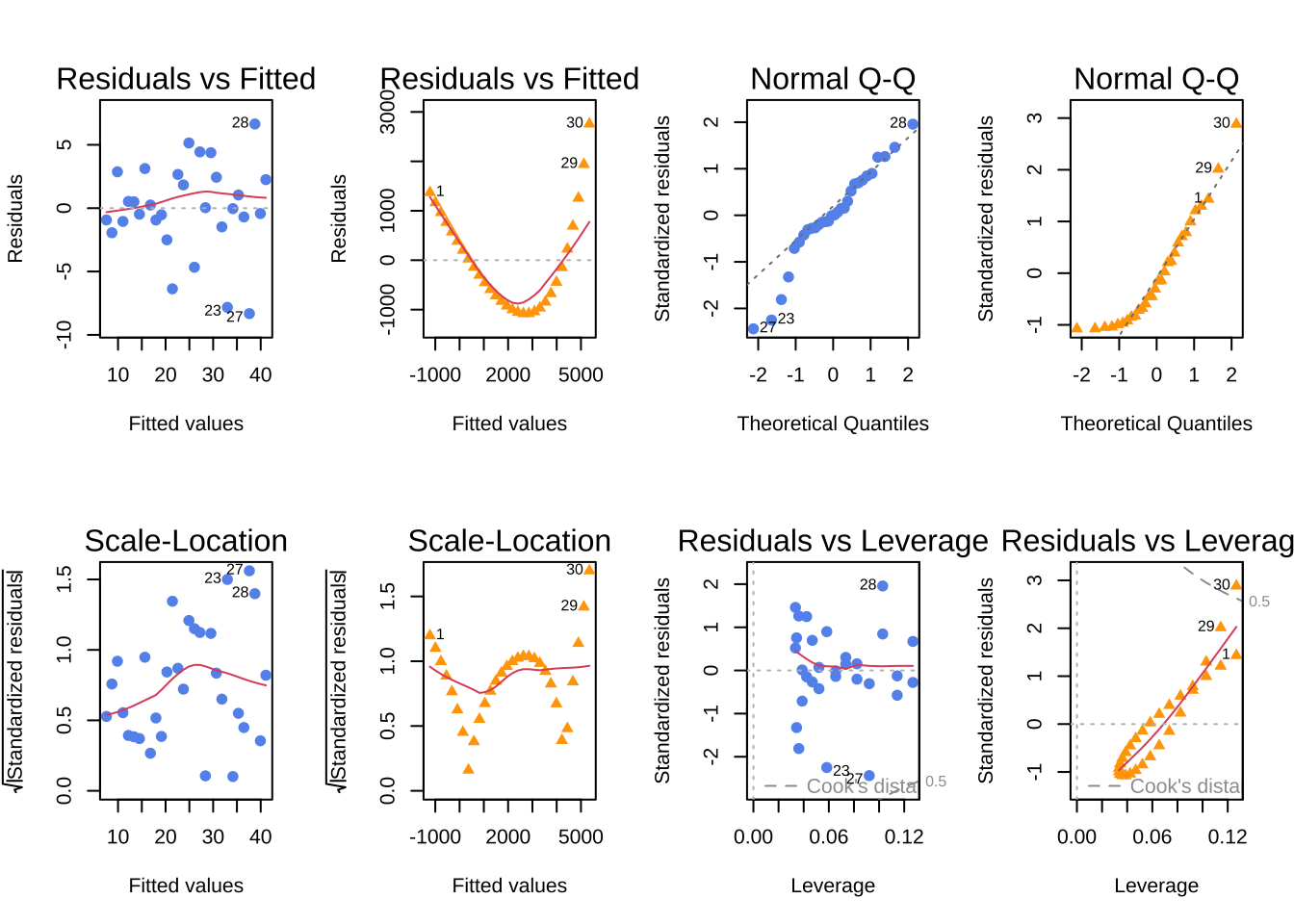

Code

dev.off()

null device 
          1

comparison plots

Code

model1_plot_noline + ex_plot_noline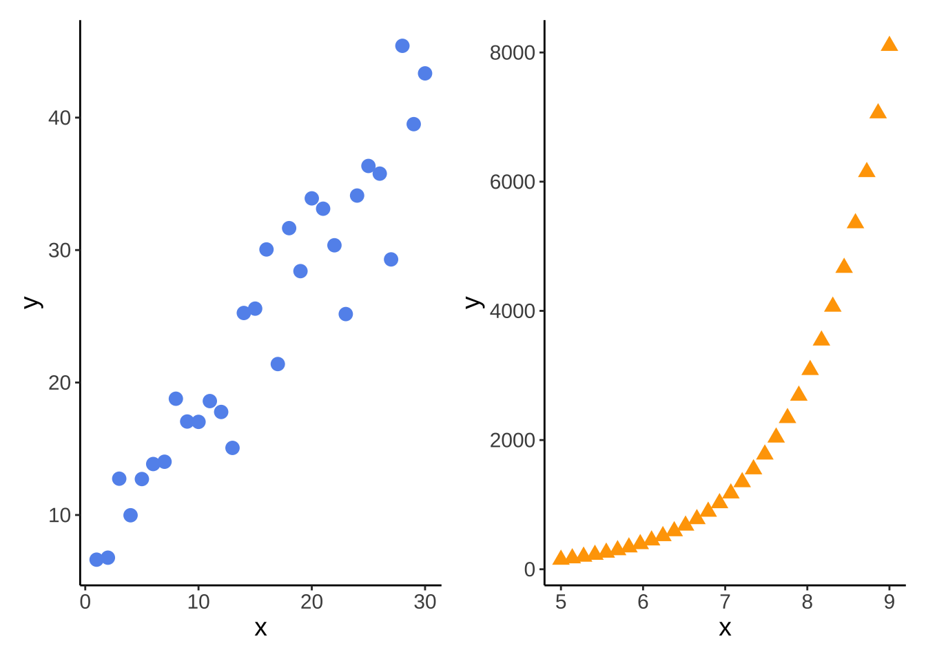

Code

model1_plot + ex_plot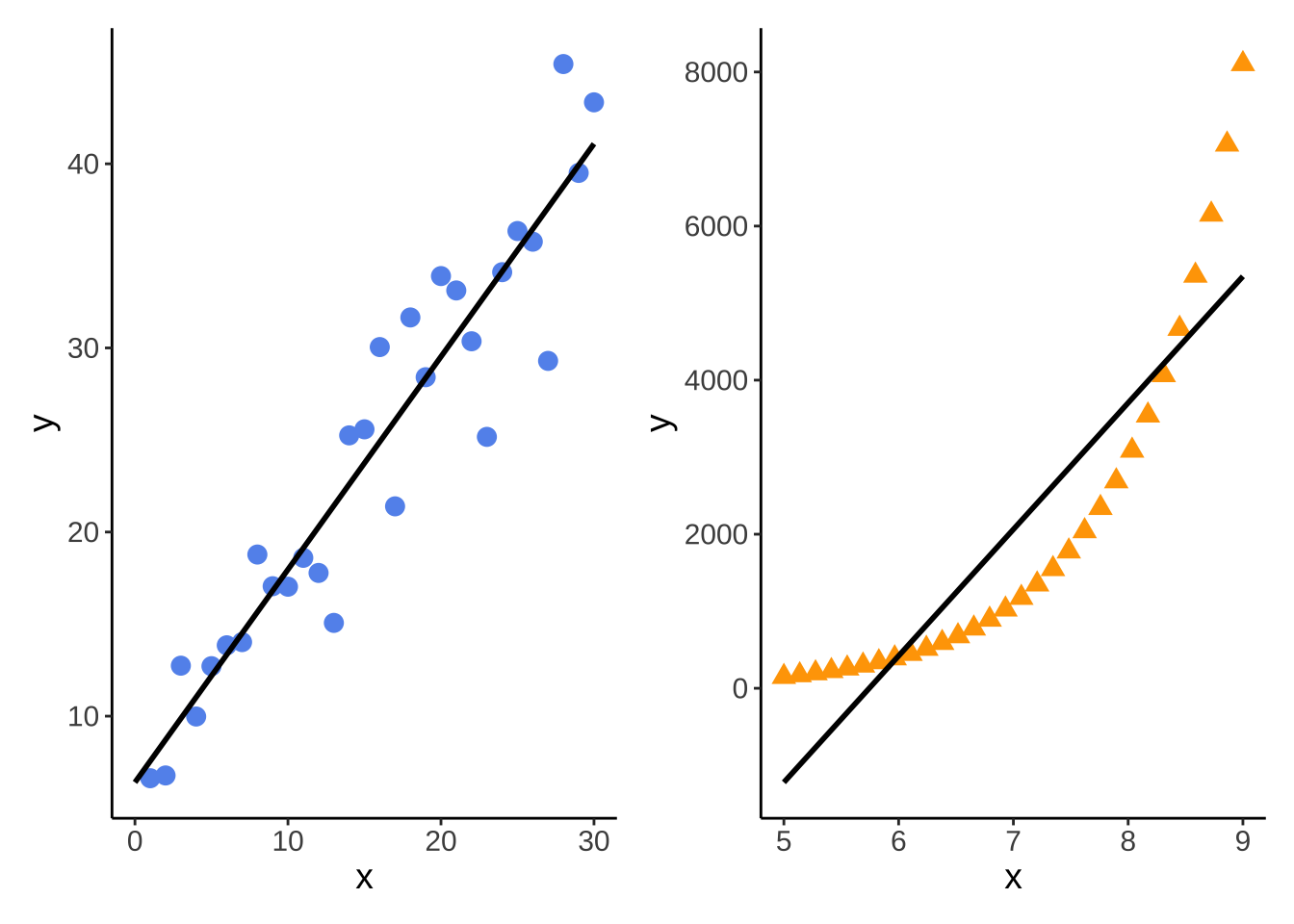

correlation?

Code

x <- x_lm
y <- y_lm

Code

cor.test(x, y, method = "pearson")


    Pearson's product-moment correlation

data:  x and y
t = 15.293, df = 28, p-value = 4.021e-15
alternative hypothesis: true correlation is not equal to 0
95 percent confidence interval:
 0.8866210 0.9737646
sample estimates:
      cor 
0.9450274

formula for Pearson’s correlation

\[ r = \frac{\sum(x_i - \bar{x})(y_i - \bar{y})}{\sqrt{\sum(x_i-\bar{x})^2}\sqrt{\sum(y_i - \bar{y})^2}} \]

test statistic for pearson correlation

\[ \begin{align} t &= \frac{r\sqrt{n - 2}}{\sqrt{1-r^2}} \\ df &= n -2 \end{align} \]

uses a t-distribution

no correlation but clear relationship

Code

x_lm <- seq(from = 1, to = 30, length.out = 50)
# y = a( x – h) 2 + k
df_para <- cbind(
  x = x_lm,
  y = 0.1*(x_lm - 15)^2 + 12
) %>% 
  as_tibble()

ggplot(df_para, aes(x = x, y = y)) +
  geom_point(size = 3) +
  theme_bw()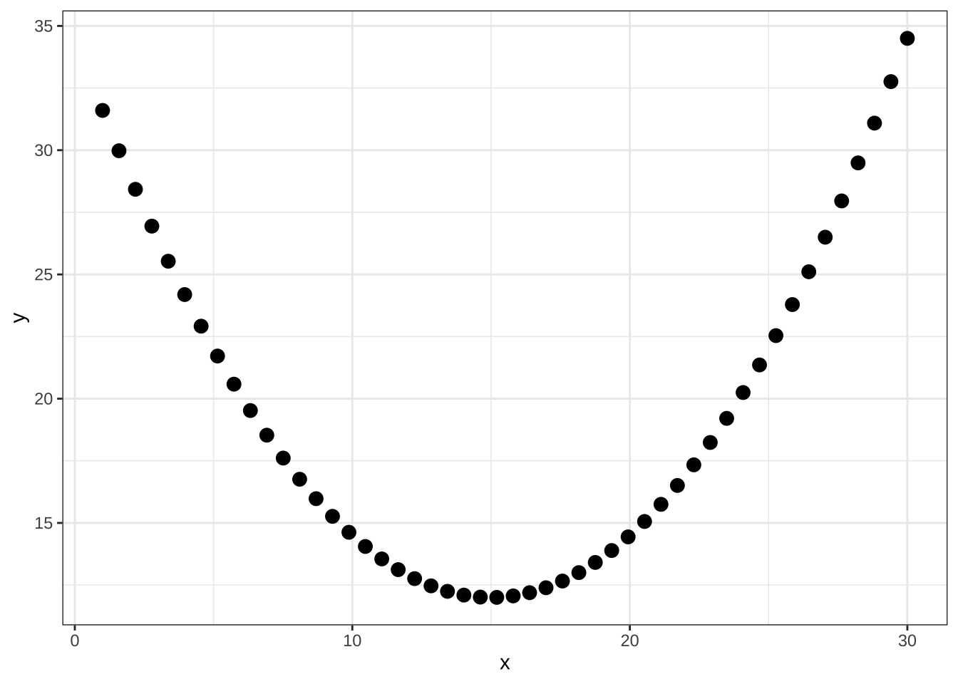

Code

cor.test(df_para$x, df_para$y, method = "pearson")


    Pearson's product-moment correlation

data:  df_para$x and df_para$y
t = 0.90749, df = 48, p-value = 0.3687
alternative hypothesis: true correlation is not equal to 0
95 percent confidence interval:
 -0.1540408  0.3939806
sample estimates:
      cor 
0.1298756

Citation

BibTeX citation:

@online{bui2023,
  author = {Bui, An},
  title = {Lecture 07 Figures},
  date = {2023-05-15},
  url = {https://an-bui.github.io/ES-193DS-W23/lecture/lecture-07_2023-05-15.html},
  langid = {en}
}

For attribution, please cite this work as:

Bui, An. 2023. “Lecture 07 Figures.” May 15, 2023. https://an-bui.github.io/ES-193DS-W23/lecture/lecture-07_2023-05-15.html.