Code

library(tidyverse)
library(palmerpenguins)
library(showtext)
library(car)
font_add_google("Lato", "Lato")
showtext_auto()
library(patchwork)
library(ggeffects)
library(performance)
library(broom)
library(flextable)
library(DHARMa)
library(GGally)
library(MuMIn)

multiple linear regression equation

\[ \begin{align} y &= \beta_0 + \beta_1x_1 + \beta_2x_2 + ... \beta_kx_k + \epsilon \end{align} \]

formulas

sum of squares for linear regression

regression (or model)

\[ SS_{reg} = \sum_{i = 1}^{n}(\hat{y} - \bar{y})^2 \]

error

\[ SS_{err} = \sum_{i = 1}^{n}(y_i - \hat{y})^2 \]

total

\[ SS_{tot} = \sum_{i = 1}^n(y_i - \bar{y}) \]

mean square

regression

\[ MS_{reg} = \frac{SS_{reg}}{1} \]

error

\[ MS_{err} = \frac{SS_{err}}{n - 2} \]

F-statistic

\[ F = \frac{MS_{reg}}{MS_{err}} \]

plant example

Code

set.seed(666)
# sample size
n <- 64
plant_df <- tibble(
  # predictor variables
  temperature = round(rnorm(n = n, mean = 28, sd = 1), digits = 1),
  light = round(rnorm(n = n, mean = 1, sd = 0.2), digits = 1),
  ph = rnorm(n = n, mean = 7, sd = 0.01),
  
  # response: growth in cm/week
  growth = light*rnorm(n = n, mean = 0.3, sd = 0.1) + temperature/round(rnorm(n = n, mean = 5, sd = 0.1))
)

Code

plant_model <- lm(growth ~ light + temperature + ph, data = plant_df)

Code

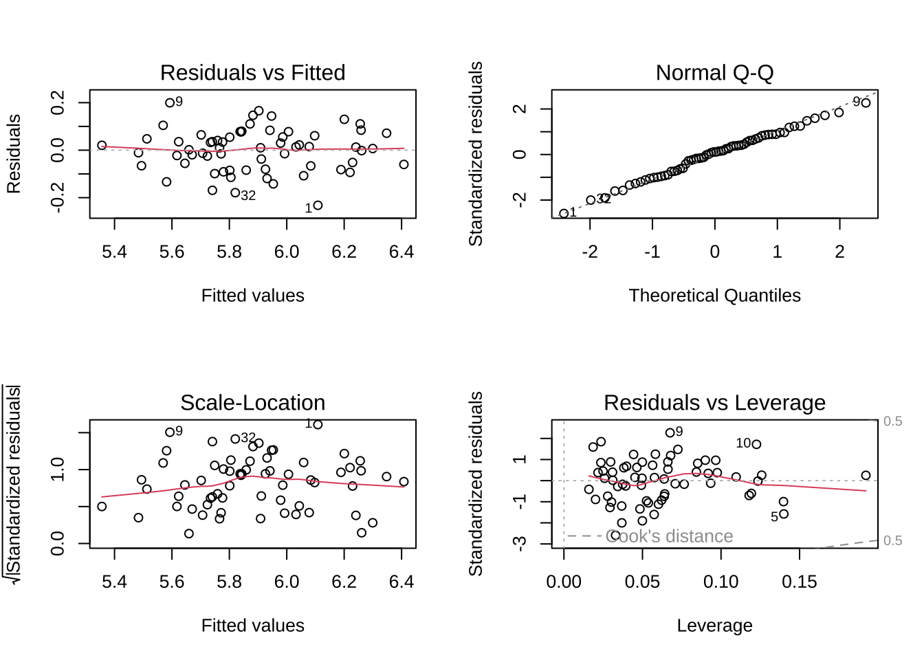
par(mfrow = c(2, 2))
plot(plant_model)

Code

check_model(plant_model)

Code

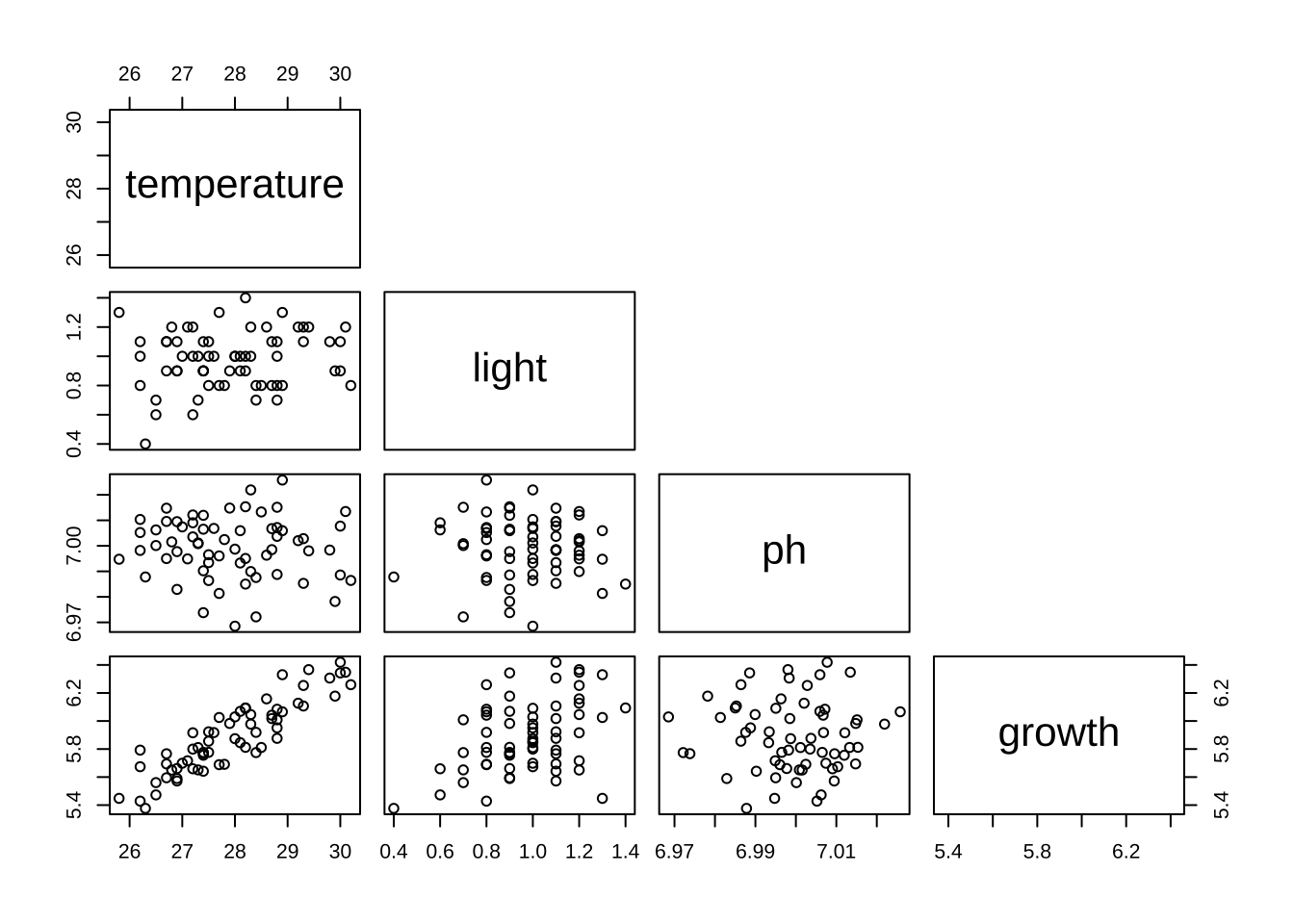
pairs(plant_df, upper.panel = NULL)

Code

ggpairs(plant_df)

Code

cor(plant_df)

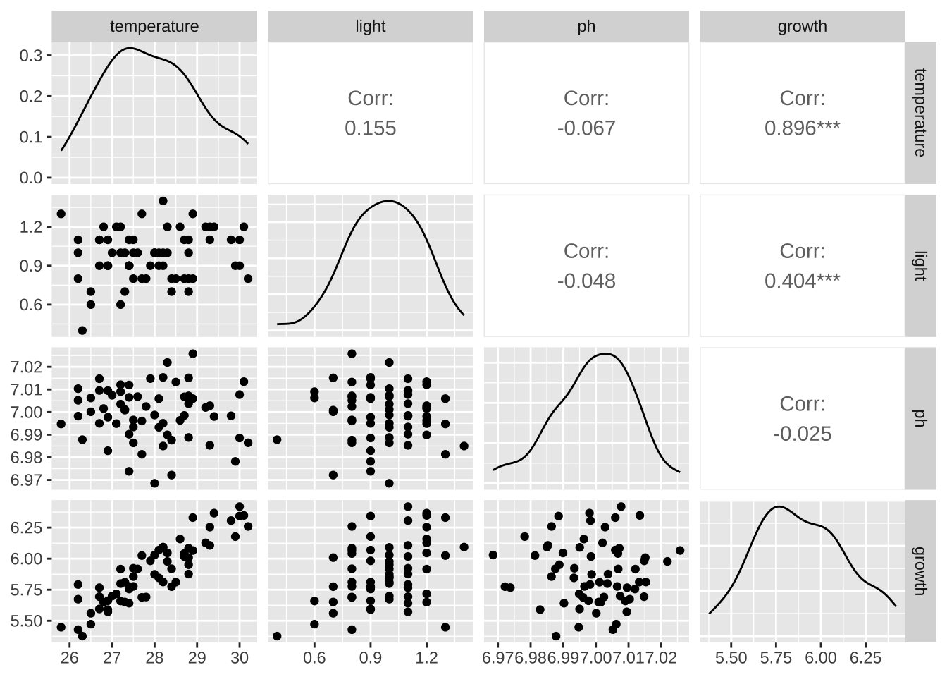
            temperature       light          ph      growth
temperature  1.00000000  0.15540780 -0.06657697  0.89551840
light        0.15540780  1.00000000 -0.04769987  0.40397013
ph          -0.06657697 -0.04769987  1.00000000 -0.02466729
growth       0.89551840  0.40397013 -0.02466729  1.00000000

Code

vif(plant_model)

      light temperature          ph 
   1.026223    1.028447    1.005897

Code

summary(plant_model)


Call:
lm(formula = growth ~ light + temperature + ph, data = plant_df)

Residuals:
     Min       1Q   Median       3Q      Max 
-0.23209 -0.06571  0.01010  0.06173  0.19950 

Coefficients:
            Estimate Std. Error t value Pr(>|t|)    
(Intercept) -6.67140    6.80194  -0.981    0.331    
light        0.35196    0.05939   5.926 1.63e-07 ***
temperature  0.19626    0.01058  18.558  < 2e-16 ***
ph           0.96241    0.96806   0.994    0.324    
---
Signif. codes:  0 '***' 0.001 '**' 0.01 '*' 0.05 '.' 0.1 ' ' 1

Residual standard error: 0.0911 on 60 degrees of freedom
Multiple R-squared:  0.8759,    Adjusted R-squared:  0.8696 
F-statistic: 141.1 on 3 and 60 DF,  p-value: < 2.2e-16

Code

anova(plant_model)

Analysis of Variance Table

Response: growth
            Df  Sum Sq Mean Sq  F value    Pr(>F)    
light        1 0.65459 0.65459  78.8700 1.567e-12 ***
temperature  1 2.85039 2.85039 343.4377 < 2.2e-16 ***
ph           1 0.00820 0.00820   0.9884    0.3241    
Residuals   60 0.49797 0.00830                       
---
Signif. codes:  0 '***' 0.001 '**' 0.01 '*' 0.05 '.' 0.1 ' ' 1

For example, temperature F-value:

Code

2.85039/0.0083

[1] 343.4205

\[ \begin{align} F &= \frac{2.85039}{0.00830} \\ &= 343.4205 \end{align} \]

frog example

generating data

Code

set.seed(666)
frog_n <- 87

df <- cbind(
  # predictor variables
  color = sample(x = c("blue", "green", "red"), size = frog_n, replace = TRUE, prob = c(0.3, 0.3, 0.3)),
  weight = (round(rnorm(n = frog_n, mean = 3, sd = 0.3), 2)),
  pattern = sample(x = c("striped", "spotted", "none"), size = frog_n, replace = TRUE, prob = c(0.3, 0.3, 0.3))
) %>% 
  as_tibble() %>% 
  mutate(weight = as.numeric(weight),
         color = as.factor(color),
         pattern = as.factor(pattern)) %>% 
  group_by(color, pattern) %>% 
  # response variable
  mutate(toxicity = case_when(
    color == "blue" & pattern == "striped" ~ rnorm(n = length(color), mean = 5, sd = 1),
    color == "blue" & pattern == "spotted" ~ rnorm(n = length(color), mean = 4, sd = 1),
    color == "green" & pattern == "striped" ~ rnorm(n = length(color), mean = 4, sd = 1),
    color == "green" & pattern == "spotted" ~ rnorm(n = length(color), mean = 3, sd = 1),
    color == "red" ~ rnorm(n = length(color), mean = 6, sd = 1),
    TRUE ~ rnorm(n = length(color), mean = 2, sd = 1)
  )) %>%
  ungroup()

plotting data

Code

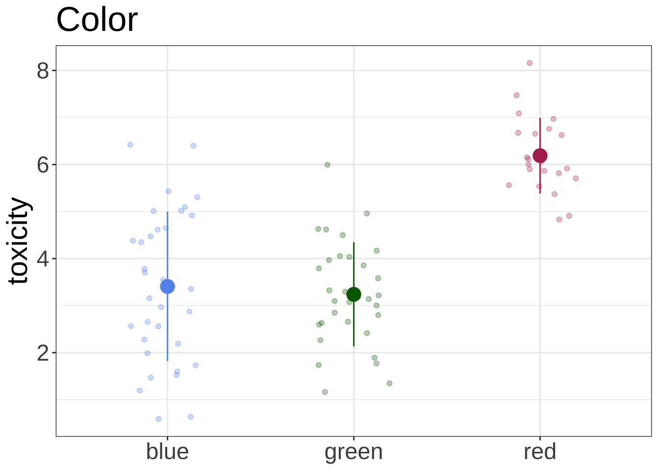
blue_col <- "cornflowerblue"
green_col <- "darkgreen"
red_col <- "maroon"

striped_col <- "grey1"
spotted_col <- "grey50"
none_col <- "grey80"

ggplot(data = df, aes(x = color, y = toxicity, color = color, fill = color)) +
  geom_jitter(width = 0.2, height = 0, alpha = 0.3) +
  scale_color_manual(values = c("blue" = blue_col, "green" = green_col, "red" = red_col)) +
  scale_fill_manual(values = c("blue" = blue_col, "green" = green_col, "red" = red_col)) +
  stat_summary(geom = "pointrange", fun = mean, fun.min = function(x) mean(x) - sd(x), fun.max = function(x) mean(x) + sd(x), shape = 21, size = 1) +
 #  geom_point(position = position_jitter(width = 0.2, height = 0, seed = 666), alpha = 0.3) +
  labs(title = "Color") +
  theme_bw() +
  theme(legend.position = "none",
        axis.title.x = element_blank(),
        text = element_text(size = 22))

Code

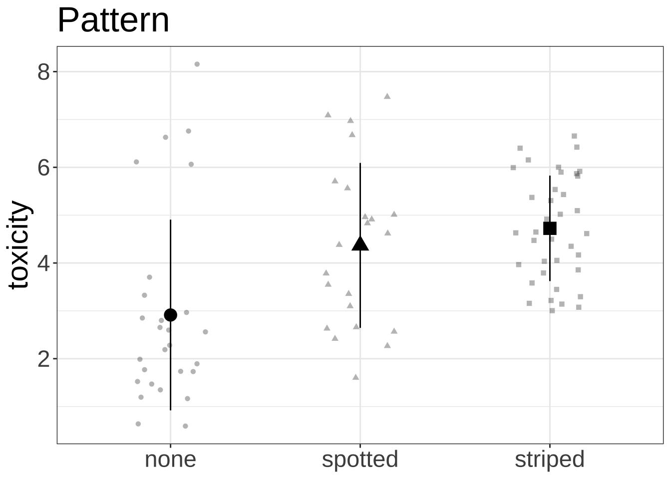
ggplot(data = df, aes(x = pattern, y = toxicity, shape = pattern)) +
  geom_jitter(width = 0.2, height = 0, alpha = 0.3) +
  # scale_color_manual(values = c("blue" = blue_col, "green" = green_col, "red" = red_col)) +
  # scale_fill_manual(values = c("striped" = striped_col, "spotted" = spotted_col, "none" = none_col)) +
  stat_summary(geom = "pointrange", fun = mean, fun.min = function(x) mean(x) - sd(x), fun.max = function(x) mean(x) + sd(x), size = 1) +
  labs(title = "Pattern") +
  theme_bw() +
  theme(legend.position = "none",
        axis.title.x = element_blank(),
        text = element_text(size = 22))

Code

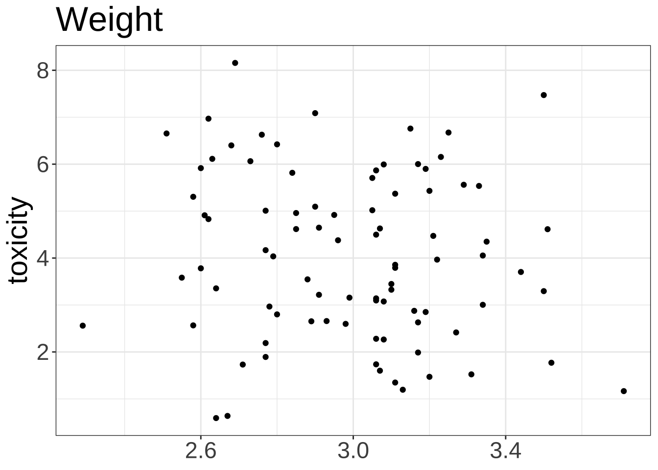
ggplot(data = df, aes(x = weight, y = toxicity)) +
  geom_point() +
  # geom_smooth(method = "lm") +
  labs(title = "Weight") +
  theme_bw() +
  theme(legend.position = "none",
        axis.title.x = element_blank(),
        text = element_text(size = 22))

Code

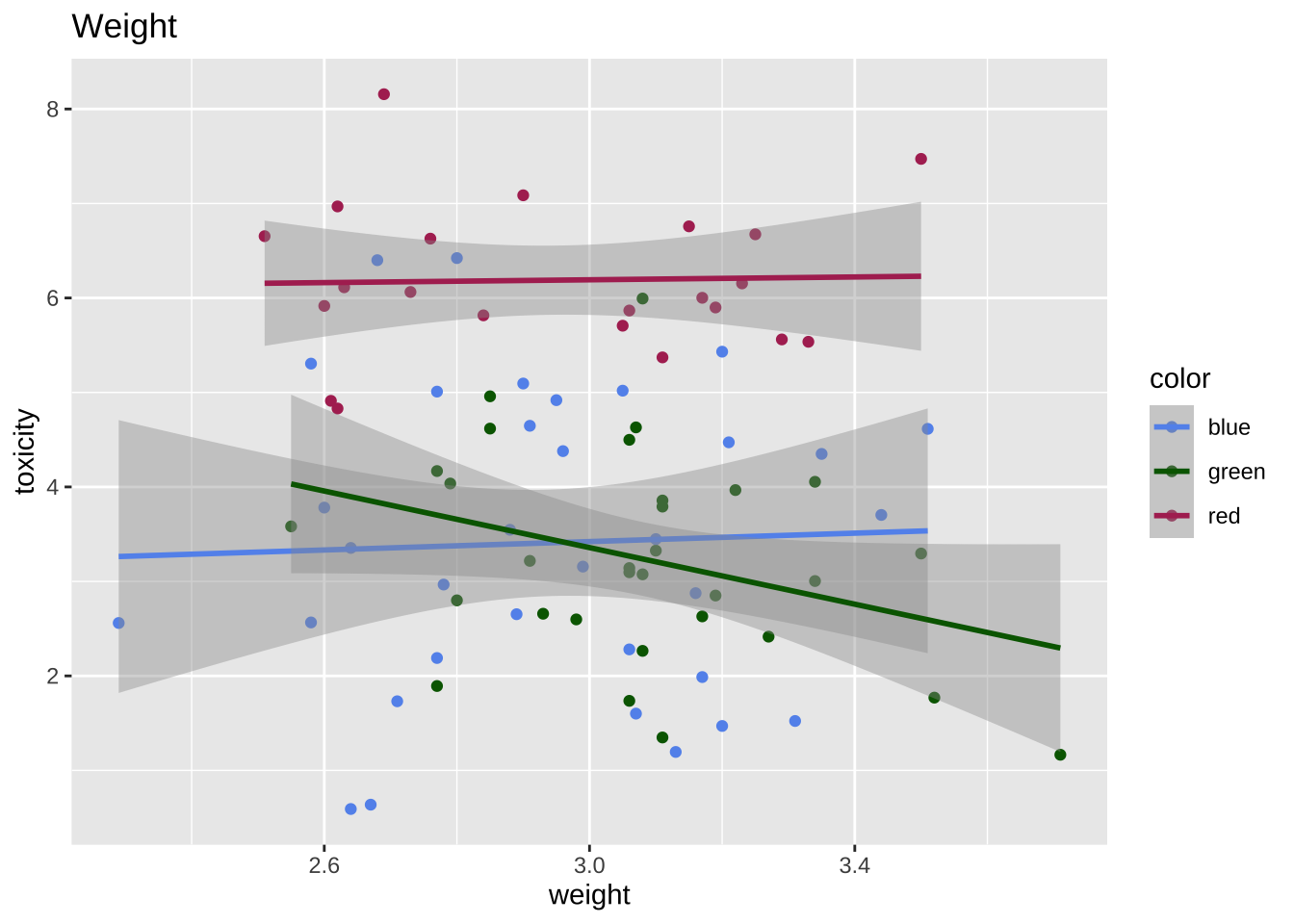
ggplot(data = df, aes(x = weight, y = toxicity, color = color)) +
  geom_point() +
  scale_color_manual(values = c("blue" = blue_col, "green" = green_col, "red" = red_col)) +
  geom_smooth(method = "lm") +
  labs(title = "Weight")

model

Code

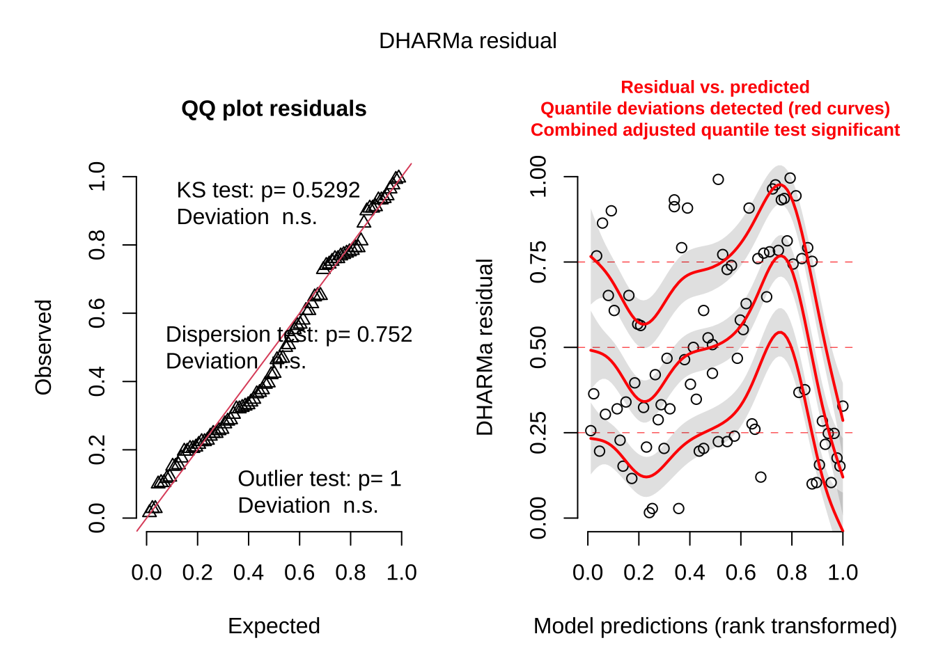
model <- lm(toxicity ~ weight + color + pattern, data = df)
simulateResiduals(model, plot = TRUE)

Object of Class DHARMa with simulated residuals based on 250 simulations with refit = FALSE . See ?DHARMa::simulateResiduals for help. 
 
Scaled residual values: 0.208 0.608 0.196 0.468 0.744 0.792 0.908 0.792 0.992 0.256 0.324 0.768 0.468 0.32 0.204 0.908 0.288 0.76 0.156 0.104 ...

diagnostics

Code

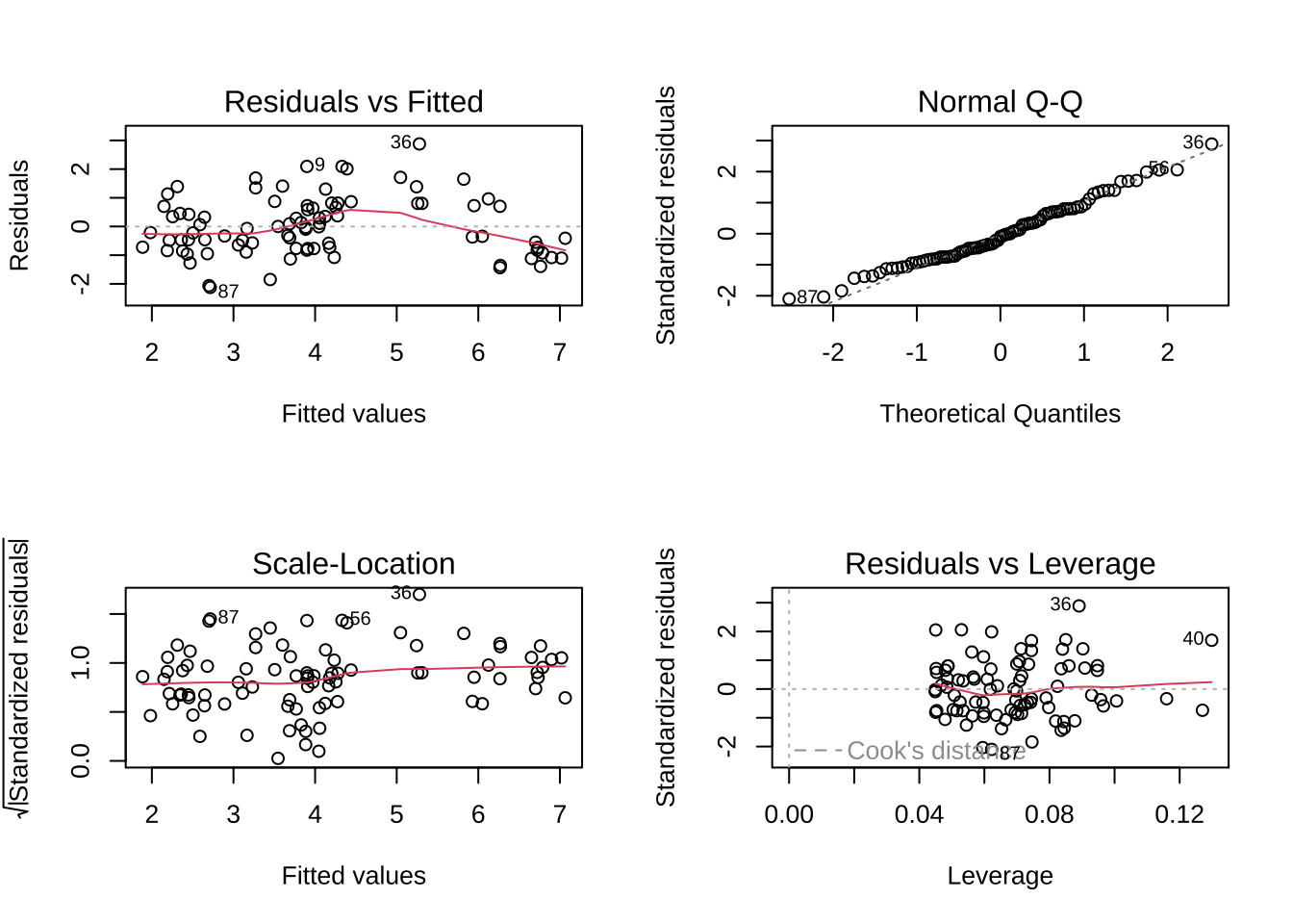
par(mfrow = c(2, 2))
plot(model)

model summary

Code

# F-statistic: 31.05 on 5 and 81 DF,  p-value: < 2.2e-16
# total SSE - SSE of residuals divided by degrees of freedom
totalSSE <- 6.932+140.09+21.63
totaldf <- 1+2+2
errorSSE <- 88
model_fstat <- (totalSSE/5)/(errorSSE/81) 
model_fstat

[1] 31.0473

Code

# for a single coefficient
weightMS <- 6.932
weightdf <- 1
errorMS <- 1.086
fvalweight <- (weightMS/weightdf)/errorMS
fvalweight

[1] 6.383057

Code

colorMS <- 70.045
colordf <- 2
fvalcolor <- (colorMS/colordf)/errorMS
fvalcolor

[1] 32.24908

Code

# residual mean sq = 1.086 (denominator)
# equation: t = 5.5 - 0.74*W - 0.97*green + 2.1*red + 0.85*spotted + 1.2*striped

Code

model_summary <- summary(model)

Anova(model)

Anova Table (Type II tests)

Response: toxicity
           Sum Sq Df F value    Pr(>F)    
weight      1.547  1  1.4194     0.237    
color     119.288  2 54.7107 9.229e-16 ***
pattern    44.843  2 20.5669 5.981e-08 ***
Residuals  88.304 81                      
---
Signif. codes:  0 '***' 0.001 '**' 0.01 '*' 0.05 '.' 0.1 ' ' 1

Code

model.sel(model)

Model selection table 
      (Intrc) color pttrn weght df   logLik  AICc delta
model   4.045     +     +     1  7 -124.095 263.6     0
Models ranked by AICc(x)

\[ \hat{y}_h \pm t_{(1-\alpha/2, n-2)}*\sqrt{MSE*(\frac{1}{n}+\frac{(x_h-\bar{x})^2}{\sum(x_i-\bar{x})^2})} \]

\[ MSE = \frac{\sum(y_i-\hat{y})^2}{n} \]

Code

tidy(model, conf.int = TRUE, conf.level = 0.95)

# A tibble: 6 × 7
  term           estimate std.error statistic  p.value conf.low conf.high
  <chr>             <dbl>     <dbl>     <dbl>    <dbl>    <dbl>     <dbl>
1 (Intercept)       4.04      1.26       3.21 1.92e- 3    1.54      6.55 
2 weight           -0.504     0.423     -1.19 2.37e- 1   -1.35      0.338
3 colorgreen       -0.289     0.267     -1.08 2.82e- 1   -0.821     0.243
4 colorred          2.59      0.290      8.91 1.17e-13    2.01      3.17 
5 patternspotted    0.952     0.303      3.14 2.34e- 3    0.349     1.55 
6 patternstriped    1.70      0.264      6.41 8.92e- 9    1.17      2.22

Code

c("lower" = model_summary$coef[2,1] - qt(0.975, df = model_summary$df[2]) * model_summary$coef[2, 2],
  "upper" = model_summary$coef[2,1] + qt(0.975, df = model_summary$df[2]) * model_summary$coef[2, 2])

     lower      upper 
-1.3451604  0.3375674

Confidence interval for a single coefficient: in words: estimate plus or minus the t-value at your confidence level * standard error

Citation

BibTeX citation:

@online{bui2023,
  author = {Bui, An},
  title = {Lecture 08 Figures},
  date = {2023-05-22},
  url = {https://an-bui.github.io/ES-193DS-W23/lecture/lecture-08_2023-05-22.html},
  langid = {en}
}

For attribution, please cite this work as:

Bui, An. 2023. “Lecture 08 Figures.” May 22, 2023. https://an-bui.github.io/ES-193DS-W23/lecture/lecture-08_2023-05-22.html.