Code

library(tidyverse)
library(showtext)
font_add_google("Lato", "Lato")
showtext_auto()
library(patchwork)
library(palmerpenguins)
library(ggeffects)
library(equatiomatic)
library(lmtest)

math notation

simple linear regression

\[ E[y_i] = a + bx_i \]

\[ var[y_i] = s^2 \]

generalized form:

\[ E[y_i] = a + bx_i \]

\[ var[y_i] = v(E[y_i]) \]

GLM structure using Gaussian example

random component

\[ Y_i \sim N(\mu_i, \sigma^2) \]

systematic component

\[ \eta_i = \sum^{p-1}_{n = 0}\beta_jx_{ij} \]

link

\[ g(\mu_i) = \eta_i \]

negative binomial example

Code

set.seed(666)
nbinom_df <- bind_cols(
  size1 = rnbinom(mu = 10, size = 1, n = 100),
  size10 = rnbinom(mu = 10, size = 10, n = 100),
  size100 = rnbinom(mu = 10, size = 100, n = 100)
)

ggplot(data.frame(x = 1:20), aes(x)) +
  stat_function(geom = "point", n = 20, fun = dnbinom, args = list(mu = 4, x = 5), size = 2) +
  stat_function(geom = "line", n = 20, fun = dnbinom, args = list(mu = 4, x = 5))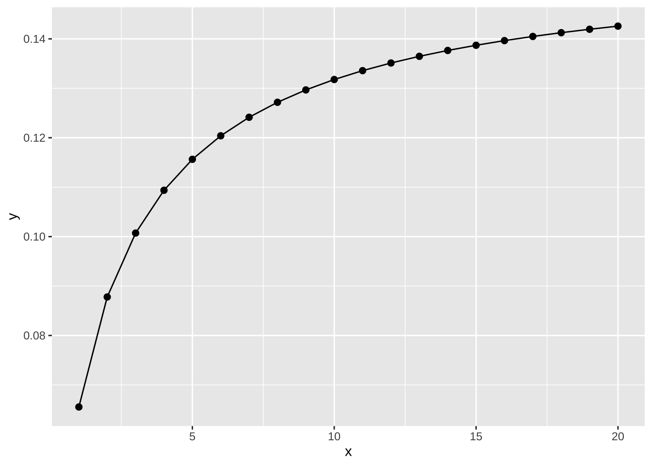

Code

size1 <- ggplot(nbinom_df, aes(x = size1)) +
  geom_histogram(bins = 8, fill = "cornflowerblue", color = "grey8") +
  scale_y_continuous(expand = c(0, 0), limits = c(0, 40)) +
  theme_classic() +
  labs(title = expression(mu~"= 10, k = 1")) +
  theme(axis.title.x = element_blank())

size10 <- ggplot(nbinom_df, aes(x = size10)) +
  geom_histogram(bins = 8, fill = "cornflowerblue", color = "grey8") +
  scale_y_continuous(expand = c(0, 0), limits = c(0, 40)) +
  theme_classic() +
  labs(title = expression(mu~"= 10, k = 10")) +
  theme(axis.title.x = element_blank())

size100 <- ggplot(nbinom_df, aes(x = size100)) +
  geom_histogram(bins = 8, fill = "cornflowerblue", color = "grey8") +
  scale_y_continuous(expand = c(0, 0), limits = c(0, 40)) +
  theme_classic() +
  labs(title = expression(mu~"= 10, k = 100")) +
  theme(axis.title.x = element_blank())

size1 + size10 + size100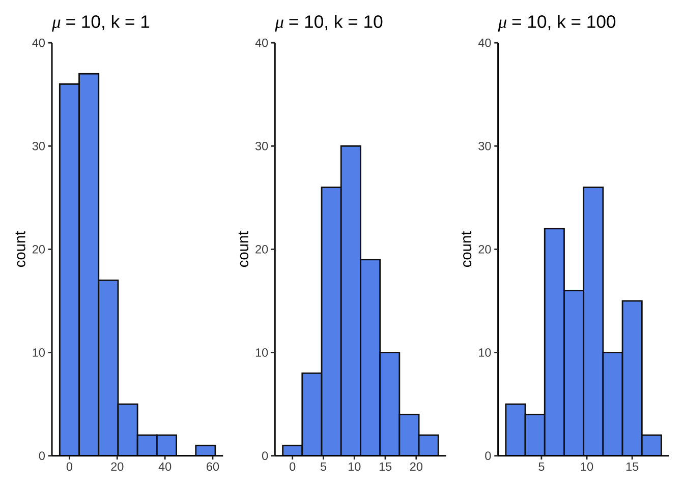

poisson example

Code

set.seed(666)
pois_df <- bind_cols(
  lambda1 = rpois(lambda = 1, n = 100),
  lambda5 = rpois(lambda = 5, n = 100),
  lambda20 = rpois(lambda = 20, n = 100)
)

lambda1 <- ggplot(pois_df, aes(x = lambda1)) +
  geom_histogram(bins = 8, fill = "darkorange", color = "grey8") +
  scale_y_continuous(expand = c(0, 0), limits = c(0, 40)) +
  theme_classic() +
  labs(title = expression(lambda~"= 1")) +
  theme(axis.title.x = element_blank())

lambda5 <- ggplot(pois_df, aes(x = lambda5)) +
  geom_histogram(bins = 8, fill = "darkorange", color = "grey8") +
  scale_y_continuous(expand = c(0, 0), limits = c(0, 40)) +
  theme_classic() +
  labs(title = expression(lambda~"= 5")) +
  theme(axis.title.x = element_blank())

lambda20 <- ggplot(pois_df, aes(x = lambda20)) +
  geom_histogram(bins = 8, fill = "darkorange", color = "grey8") +
  scale_y_continuous(expand = c(0, 0), limits = c(0, 40)) +
  theme_classic() +
  labs(title = expression(lambda~"= 20")) +
  theme(axis.title.x = element_blank())

lambda1 + lambda5 + lambda20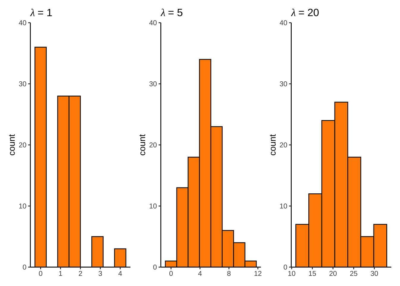

simpson’s paradox

Code

bill_model <- lm(bill_length_mm ~ bill_depth_mm, data = penguins)

par(mfrow = c(2, 2))
plot(bill_model)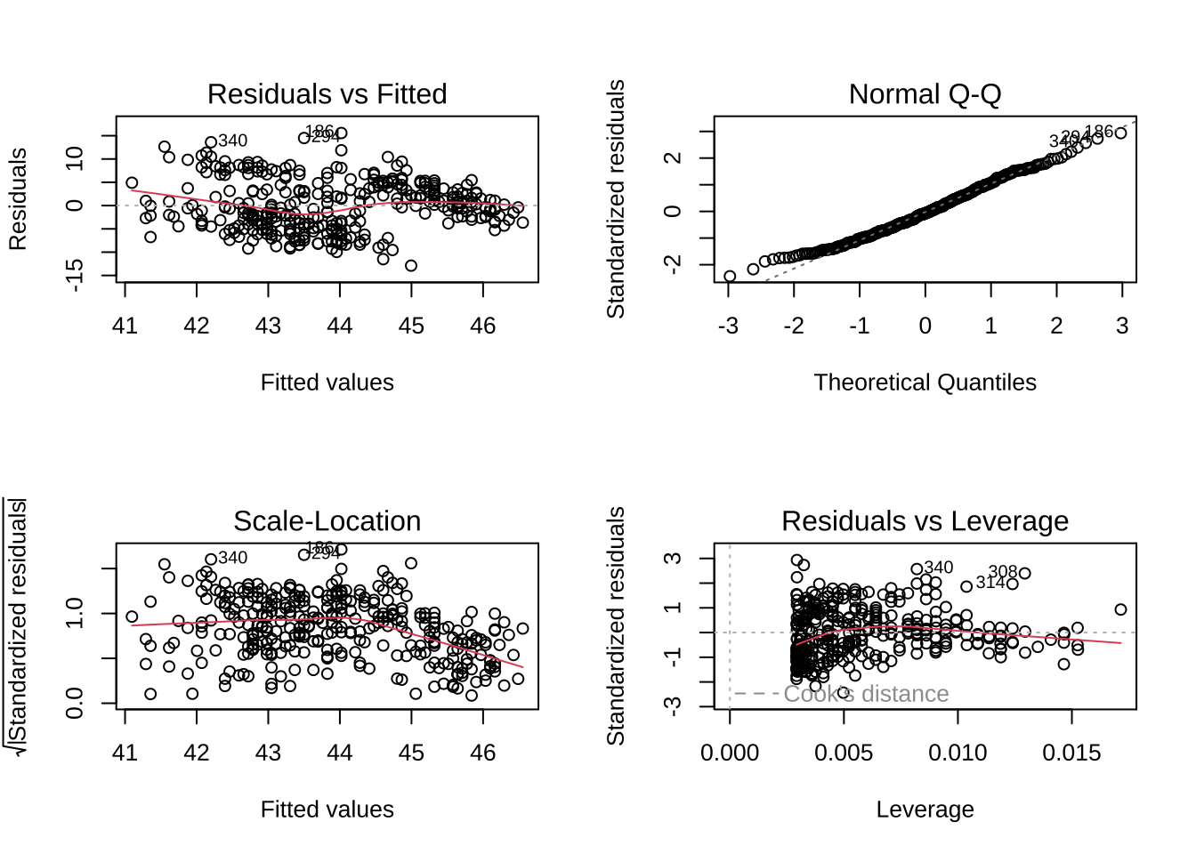

Code

summary(bill_model)


Call:
lm(formula = bill_length_mm ~ bill_depth_mm, data = penguins)

Residuals:
     Min       1Q   Median       3Q      Max 
-12.8949  -3.9042  -0.3772   3.6800  15.5798 

Coefficients:
              Estimate Std. Error t value Pr(>|t|)    
(Intercept)    55.0674     2.5160  21.887  < 2e-16 ***
bill_depth_mm  -0.6498     0.1457  -4.459 1.12e-05 ***
---
Signif. codes:  0 '***' 0.001 '**' 0.01 '*' 0.05 '.' 0.1 ' ' 1

Residual standard error: 5.314 on 340 degrees of freedom
  (2 observations deleted due to missingness)
Multiple R-squared:  0.05525,   Adjusted R-squared:  0.05247 
F-statistic: 19.88 on 1 and 340 DF,  p-value: 1.12e-05

Code

confint(bill_model)

                   2.5 %     97.5 %
(Intercept)   50.1185795 60.0161600
bill_depth_mm -0.9364867 -0.3631844

Code

bill_model_preds <- ggpredict(bill_model, terms = "bill_depth_mm")

model_plot <- ggplot(penguins, aes(x = bill_depth_mm, y = bill_length_mm)) +
  geom_point() +
  geom_line(data = bill_model_preds, aes(x = x, y = predicted), color = "blue", linewidth = 2) +
  geom_ribbon(data = bill_model_preds, aes(x = x, y = predicted, ymin = conf.low, ymax = conf.high), alpha = 0.2) +
  theme_classic() +
  labs(x = "Bill depth (mm)", y = "Bill length (mm)")

\[ length = -0.65*depth + 55.07 \]

Code

bill_model2 <- lm(bill_length_mm ~ bill_depth_mm*species, data = penguins)
par(mfrow = c(2, 2))
plot(bill_model2)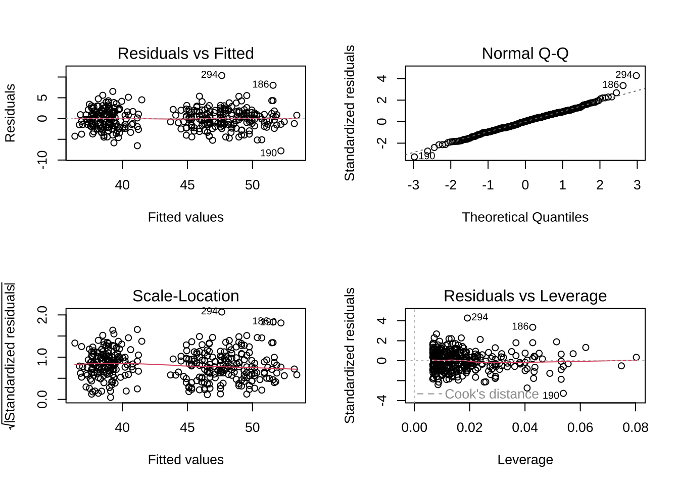

Code

summary(bill_model2)


Call:
lm(formula = bill_length_mm ~ bill_depth_mm * species, data = penguins)

Residuals:
    Min      1Q  Median      3Q     Max 
-7.7888 -1.5415  0.0575  1.5873 10.3590 

Coefficients:
                               Estimate Std. Error t value Pr(>|t|)    
(Intercept)                     23.0681     3.0165   7.647 2.18e-13 ***
bill_depth_mm                    0.8570     0.1641   5.224 3.08e-07 ***
speciesChinstrap                -9.6402     5.7154  -1.687 0.092590 .  
speciesGentoo                   -5.8386     4.5353  -1.287 0.198850    
bill_depth_mm:speciesChinstrap   1.0651     0.3100   3.435 0.000666 ***
bill_depth_mm:speciesGentoo      1.1637     0.2789   4.172 3.84e-05 ***
---
Signif. codes:  0 '***' 0.001 '**' 0.01 '*' 0.05 '.' 0.1 ' ' 1

Residual standard error: 2.445 on 336 degrees of freedom
  (2 observations deleted due to missingness)
Multiple R-squared:  0.8024,    Adjusted R-squared:  0.7995 
F-statistic: 272.9 on 5 and 336 DF,  p-value: < 2.2e-16

Code

lrtest(bill_model2)

Likelihood ratio test

Model 1: bill_length_mm ~ bill_depth_mm * species
Model 2: bill_length_mm ~ 1
  #Df   LogLik Df  Chisq Pr(>Chisq)    
1   7  -787.97                         
2   2 -1065.28 -5 554.62  < 2.2e-16 ***
---
Signif. codes:  0 '***' 0.001 '**' 0.01 '*' 0.05 '.' 0.1 ' ' 1

Code

anova(bill_model2)

Analysis of Variance Table

Response: bill_length_mm
                       Df Sum Sq Mean Sq F value    Pr(>F)    
bill_depth_mm           1  561.6   561.6  93.965 < 2.2e-16 ***
species                 2 7460.3  3730.2 624.151 < 2.2e-16 ***
bill_depth_mm:species   2  134.3    67.1  11.232 1.898e-05 ***
Residuals             336 2008.1     6.0                      
---
Signif. codes:  0 '***' 0.001 '**' 0.01 '*' 0.05 '.' 0.1 ' ' 1

Code

waldtest(bill_model2)

Wald test

Model 1: bill_length_mm ~ bill_depth_mm * species
Model 2: bill_length_mm ~ 1
  Res.Df Df      F    Pr(>F)    
1    336                        
2    341 -5 272.95 < 2.2e-16 ***
---
Signif. codes:  0 '***' 0.001 '**' 0.01 '*' 0.05 '.' 0.1 ' ' 1

Code

plot(ggpredict(bill_model2, terms = c("bill_depth_mm", "species")), add.data = TRUE)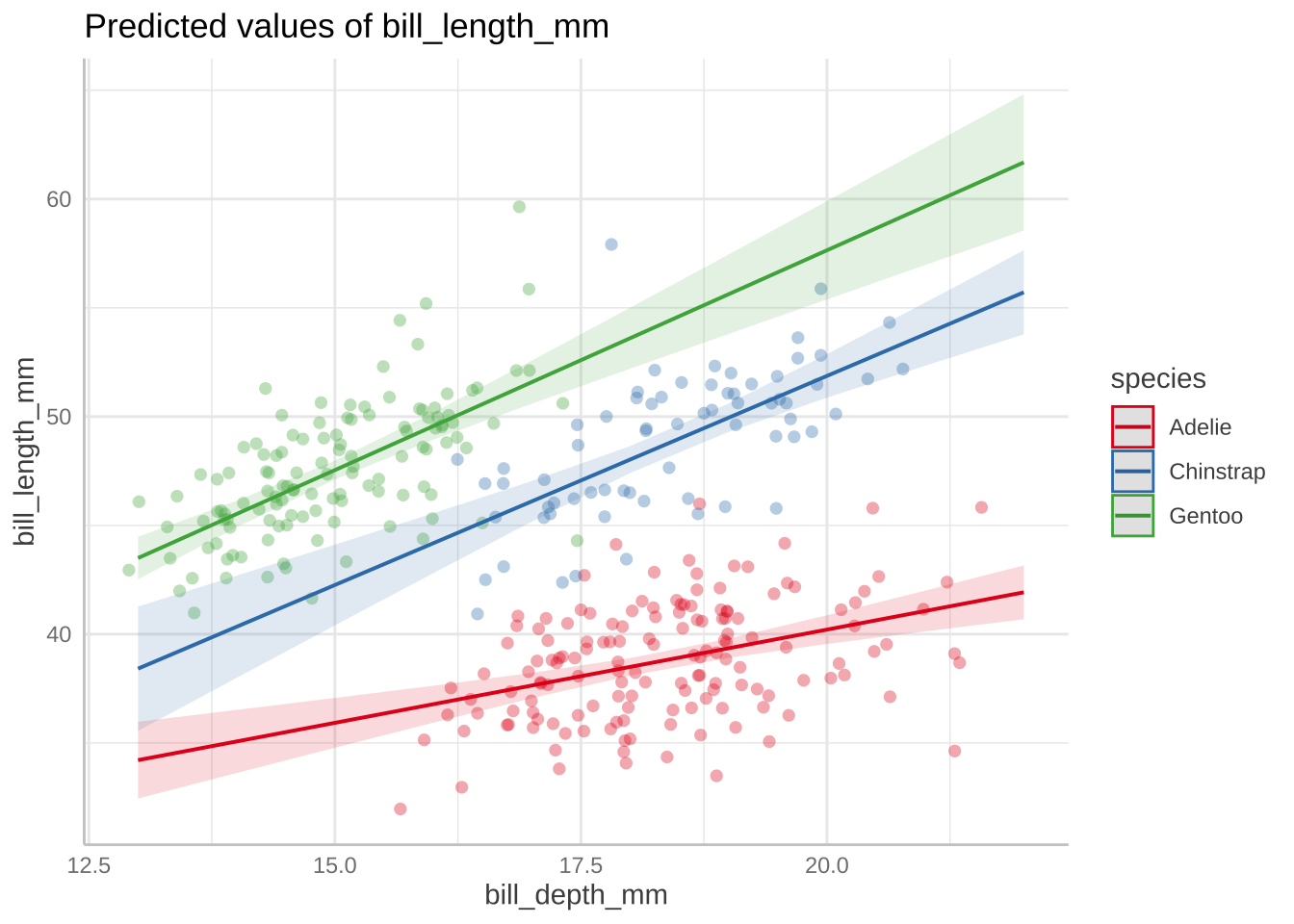

Code

bill_model2_preds <- ggpredict(bill_model2, terms = c("bill_depth_mm", "species"))

model2_plot <- ggplot(penguins, aes(x = bill_depth_mm, y = bill_length_mm)) +
  geom_point(aes(color = species)) +
  geom_line(data = bill_model2_preds, aes(x = x, y = predicted, color = group), linewidth = 2) +
  geom_ribbon(data = bill_model2_preds, aes(x = x, y = predicted, ymin = conf.low, ymax = conf.high, fill = group), alpha = 0.2) +
  scale_color_manual(values = c("cornflowerblue", "darkgreen", "darkorange")) +
  scale_fill_manual(values = c("cornflowerblue", "darkgreen", "darkorange")) +
  theme_classic() +
  labs(x = "Bill depth (mm)", y = "Bill length (mm)",
       color = "Species", fill = "Species") +
  theme(legend.position = c(0.2, 0.8))

model_plot + model2_plot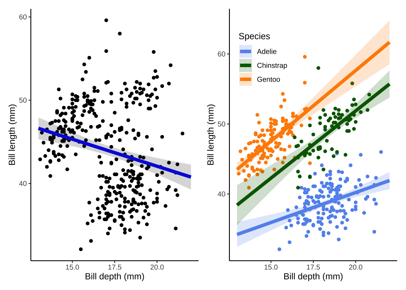

Code

extract_eq(bill_model)

\[ \operatorname{bill\_length\_mm} = \alpha + \beta_{1}(\operatorname{bill\_depth\_mm}) + \epsilon \]

\[ \operatorname{bill\_length\_mm} = \alpha + \beta_{1}(\operatorname{bill\_depth\_mm}) + \beta_{2}(\operatorname{species}_{\operatorname{Chinstrap}}) + \beta_{3}(\operatorname{species}_{\operatorname{Gentoo}}) + \beta_{4}(\operatorname{bill\_depth\_mm} \times \operatorname{species}_{\operatorname{Chinstrap}}) + \beta_{5}(\operatorname{bill\_depth\_mm} \times \operatorname{species}_{\operatorname{Gentoo}}) + \epsilon \]

\[ \operatorname{bill\_length\_mm} = \alpha + \beta_{1}(\operatorname{bill\_depth\_mm}) + \epsilon \]

Citation

BibTeX citation:

@online{bui2023,
  author = {Bui, An},
  title = {Lecture 10 Figures},
  date = {2023-06-05},
  url = {https://an-bui.github.io/ES-193DS-W23/lecture/lecture-10_2023-06-05.html},
  langid = {en}
}

For attribution, please cite this work as:

Bui, An. 2023. “Lecture 10 Figures.” June 5, 2023. https://an-bui.github.io/ES-193DS-W23/lecture/lecture-10_2023-06-05.html.