0. set up

Code

library(tidyverse)

── Attaching core tidyverse packages ──────────────────────── tidyverse 2.0.0 ──
✔ dplyr     1.1.0     ✔ readr     2.1.4
✔ forcats   1.0.0     ✔ stringr   1.5.0
✔ ggplot2   3.4.1     ✔ tibble    3.2.0
✔ lubridate 1.9.2     ✔ tidyr     1.3.0
✔ purrr     1.0.1     
── Conflicts ────────────────────────────────────────── tidyverse_conflicts() ──
✖ dplyr::filter() masks stats::filter()
✖ dplyr::lag()    masks stats::lag()
ℹ Use the ]8;;http://conflicted.r-lib.org/conflicted package]8;; to force all conflicts to become errors

Code

library(palmerpenguins)

1. Basic data exploration and summarizing

a. Review

Find the mean and standard deviation flipper length and bill length for each penguin species on Biscoe and Dream islands.

Code

penguin_subset <- penguins %>% 
  group_by(island, species) %>% 
  filter(island %in% c("Biscoe", "Dream")) %>% 
  summarize(mean_flip = mean(flipper_length_mm, na.rm = TRUE),
            sd_flip = sd(flipper_length_mm, na.rm = TRUE),
            mean_bill = mean(bill_length_mm, na.rm = TRUE),
            sd_bill = sd(bill_length_mm, na.rm = TRUE))

`summarise()` has grouped output by 'island'. You can override using the
`.groups` argument.

Code

penguin_subset

# A tibble: 4 × 6
# Groups:   island [2]
  island species   mean_flip sd_flip mean_bill sd_bill
  <fct>  <fct>         <dbl>   <dbl>     <dbl>   <dbl>
1 Biscoe Adelie         189.    6.73      39.0    2.48
2 Biscoe Gentoo         217.    6.48      47.5    3.08
3 Dream  Adelie         190.    6.59      38.5    2.47
4 Dream  Chinstrap      196.    7.13      48.8    3.34

b. New functions: `count()`, `mutate()`, `case_when()`

More functions to add to your tidyverse toolkit:

`count()`

Code

# new object names penguin_count from penguins
penguin_count <- penguins %>% 
  # group by island and species
  group_by(island, species) %>% 
  # count function counts number of rows (i.e. observations)
  count()

penguin_count

# A tibble: 5 × 3
# Groups:   island, species [5]
  island    species       n
  <fct>     <fct>     <int>
1 Biscoe    Adelie       44
2 Biscoe    Gentoo      124
3 Dream     Adelie       56
4 Dream     Chinstrap    68
5 Torgersen Adelie       52

`mutate()` + `case_when()`

First, remember how we calculated mean body mass across penguin species last week:

Code

penguins %>% 
  group_by(species) %>% 
  summarize(mean_body_mass = mean(body_mass_g, na.rm = TRUE))

# A tibble: 3 × 2
  species   mean_body_mass
  <fct>              <dbl>
1 Adelie             3701.
2 Chinstrap          3733.
3 Gentoo             5076.

mutate() creates a new column, while case_when() within mutate() allows you to tell R, “in the case when…”. For example:

Code

# create new object called penguin_newcol from penguins
penguin_newcol <- penguins %>% 
  # group by species
  group_by(species) %>% 
  # make a new column called body_mass_cat
  mutate(body_mass_cat = case_when(
    # in the case when year matches 2007, put "first"
    year == 2007 ~ "first", 
    # in the case when year matches 2008, put "second"
    year == 2008 ~ "second",
    # in the case when year matches 2009, put "third"
    year == 2009 ~ "third"
  ))

penguin_newcol

# A tibble: 344 × 9
# Groups:   species [3]
   species island    bill_length_mm bill_d…¹ flipp…² body_…³ sex    year body_…⁴
   <fct>   <fct>              <dbl>    <dbl>   <int>   <int> <fct> <int> <chr>  
 1 Adelie  Torgersen           39.1     18.7     181    3750 male   2007 first  
 2 Adelie  Torgersen           39.5     17.4     186    3800 fema…  2007 first  
 3 Adelie  Torgersen           40.3     18       195    3250 fema…  2007 first  
 4 Adelie  Torgersen           NA       NA        NA      NA <NA>   2007 first  
 5 Adelie  Torgersen           36.7     19.3     193    3450 fema…  2007 first  
 6 Adelie  Torgersen           39.3     20.6     190    3650 male   2007 first  
 7 Adelie  Torgersen           38.9     17.8     181    3625 fema…  2007 first  
 8 Adelie  Torgersen           39.2     19.6     195    4675 male   2007 first  
 9 Adelie  Torgersen           34.1     18.1     193    3475 <NA>   2007 first  
10 Adelie  Torgersen           42       20.2     190    4250 <NA>   2007 first  
# … with 334 more rows, and abbreviated variable names ¹bill_depth_mm,
#   ²flipper_length_mm, ³body_mass_g, ⁴body_mass_cat

2. Review: rendering (Quarto) and knitting (RMarkdown)

3. Review: how to use `ggplot`

Remember that making a plot using {ggplot} takes 3 important parts:
1. the ggplot() call: you’re telling R that you want to use ggplot on a specific data frame
2. the aes() call: within the ggplot() call, you’re telling R which columns contain the x- and y- axes
3. the geom_() call: you’re telling R what kind of plot you want to make.

4. Exploratory data visualization

Usually, calculating the central tendency or data spread can only go so far. To communicate effectively, we can represent these two characteristics of our data set visually. There are a few ways to do this:
- box plot (aka box and whisker plot)
- violin plot
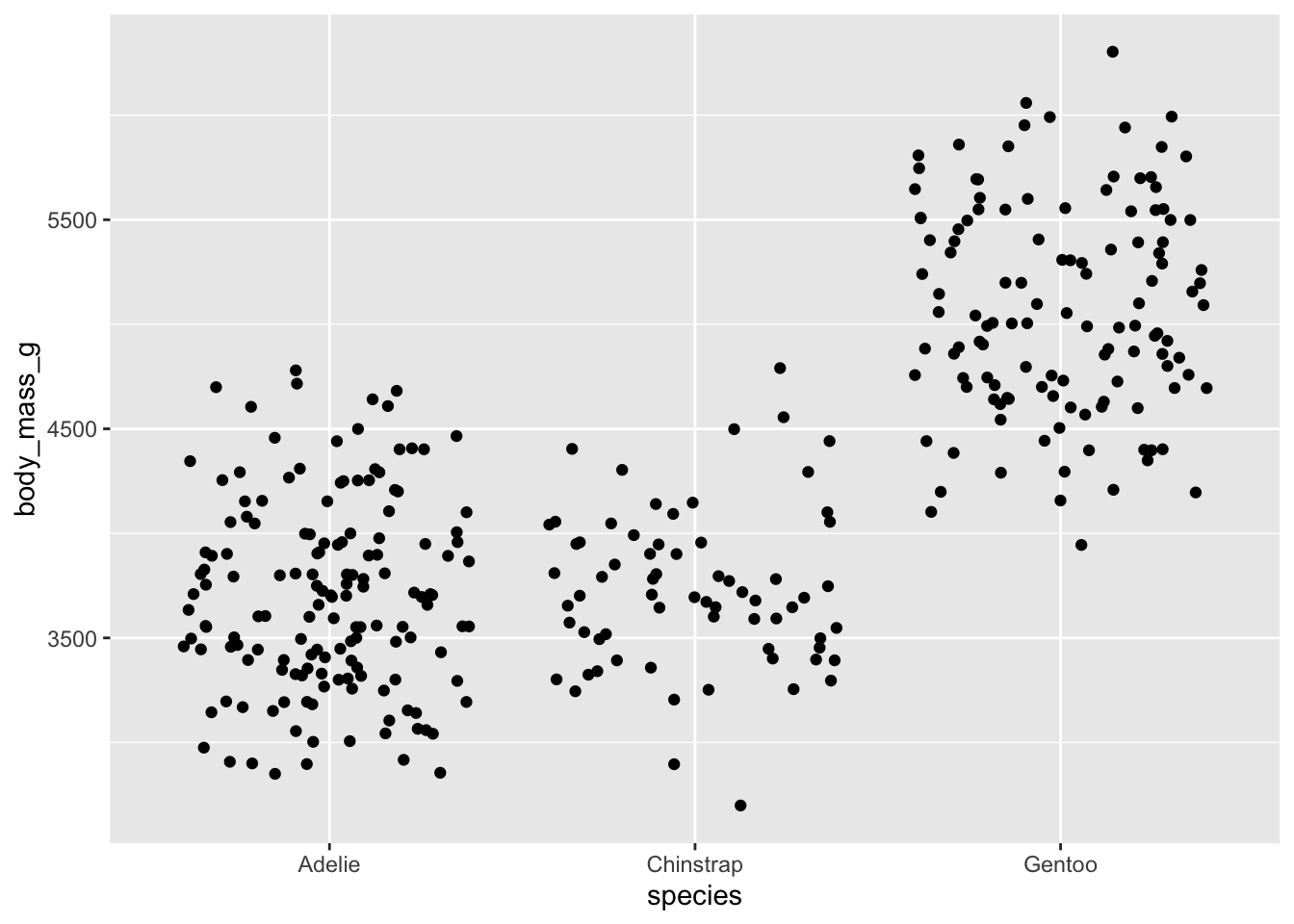
- jitter plot
- points with bars
- some combination of the above
- some other form (e.g. beeswarm)

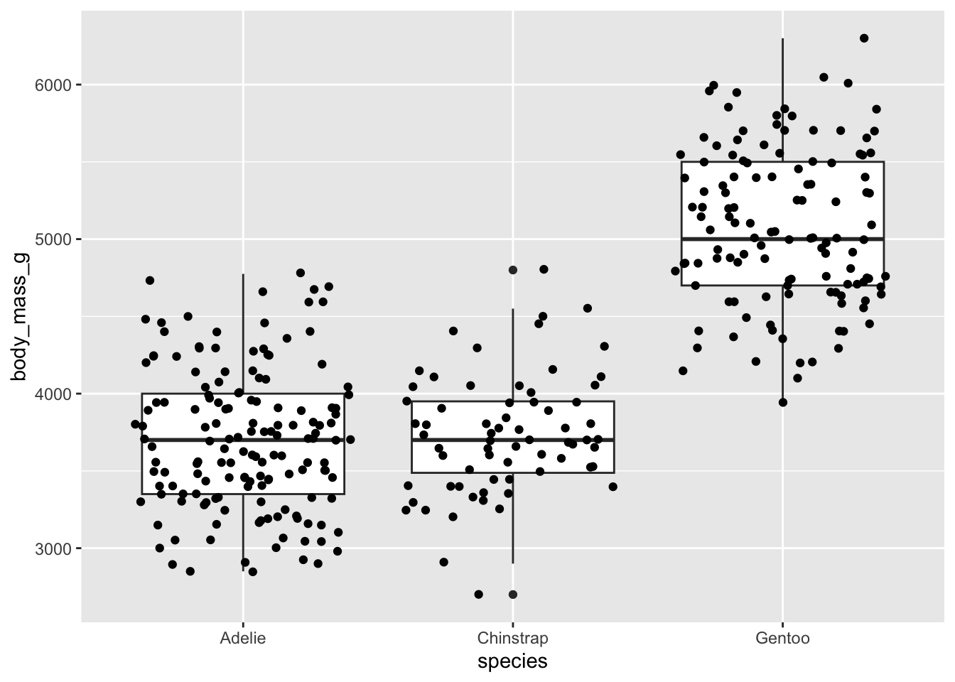
i. box plots

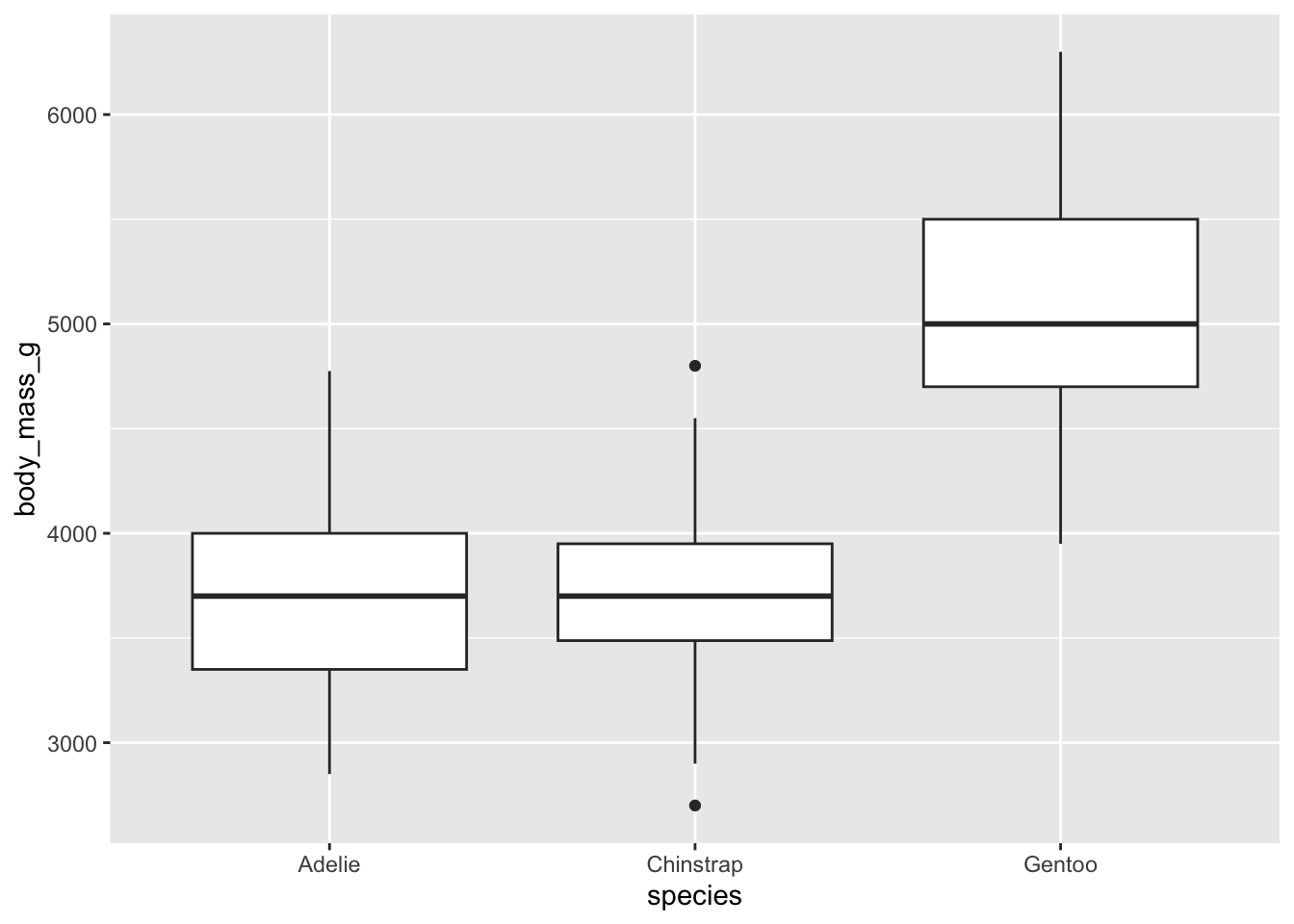
For example, let’s make a box plot of body masses for the different penguin species.

Code

ggplot(data = penguins, aes(x = species, y = body_mass_g)) +
  geom_boxplot()

Warning: Removed 2 rows containing non-finite values (`stat_boxplot()`).

Box plots are the most common way of representing central tendency and spread, but they’re not easy to parse. They usually include 1) the median, 2) the 25th quartile (median of bottom half of dataset), 3) the 75th quartile (median of top half of data set), and 4) the 1.5*inter-quartile range (distance between lower and upper quartiles). If there are any outliers, they’ll be represented as dots.

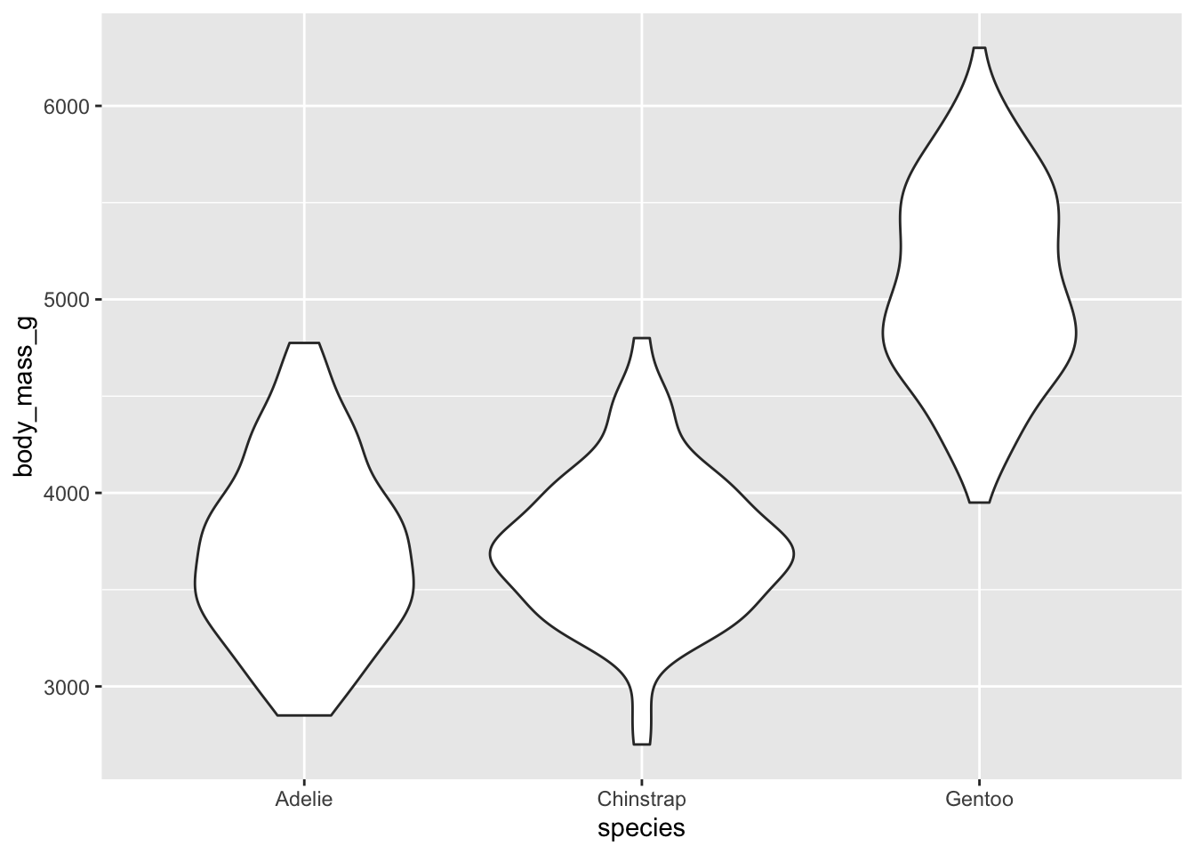
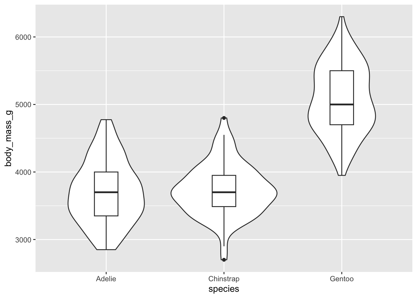
ii. violin plots

Violin plots show a symmetrical shape, and the width is based on the number of points at that particular value.

Code

ggplot(data = penguins, aes(x = species, y = body_mass_g)) +
  geom_violin()

Warning: Removed 2 rows containing non-finite values (`stat_ydensity()`).

iii. jitter plot

Jitter plots are a random smattering of points in a cloud, but the y-axis position corresponds to the real value.

Code

ggplot(data = penguins, aes(x = species, y = body_mass_g)) +
  geom_jitter()

Warning: Removed 2 rows containing missing values (`geom_point()`).

iv. points with bars

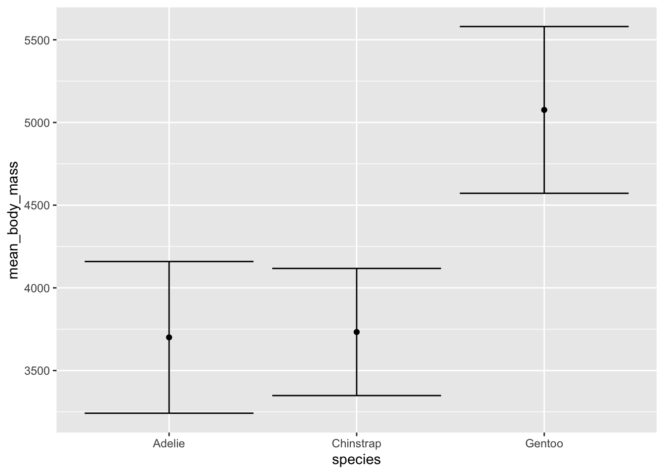
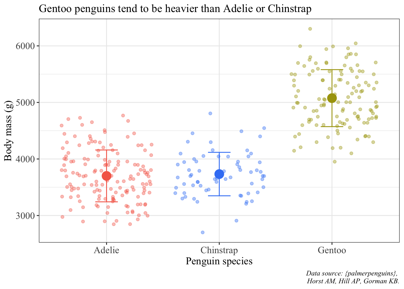
You can also represent central tendency and spread using a single point to represent the mean and bars to represent standard deviation. First, create a data frame called penguin_summary and calculate the mean and standard deviation mass for the three penguin species.

Code

penguin_summary <- penguins %>% 
  group_by(species) %>% 
  summarize(mean_body_mass = mean(body_mass_g, na.rm = TRUE),
            sd_body_mass = sd(body_mass_g, na.rm = TRUE))

Code

ggplot(data = penguin_summary, aes(x = species, y = mean_body_mass)) +
  geom_point() +
  geom_errorbar(aes(ymin = mean_body_mass - sd_body_mass, 
                    ymax = mean_body_mass + sd_body_mass))

v. some combination of the above

There are some common combinations of the above plots, for example:

violin plot with boxplot

Code

ggplot(data = penguins, aes(x = species, y = body_mass_g)) +
  geom_violin() +
  # width argument controls boxplot width
  geom_boxplot(width = 0.2)

Warning: Removed 2 rows containing non-finite values (`stat_ydensity()`).

Warning: Removed 2 rows containing non-finite values (`stat_boxplot()`).

boxplot with jittered points

Code

ggplot(data = penguins, aes(x = species, y = body_mass_g)) +
  geom_boxplot() +
  geom_jitter()

Warning: Removed 2 rows containing non-finite values (`stat_boxplot()`).

Warning: Removed 2 rows containing missing values (`geom_point()`).

4. Adjusting `ggplot` defaults

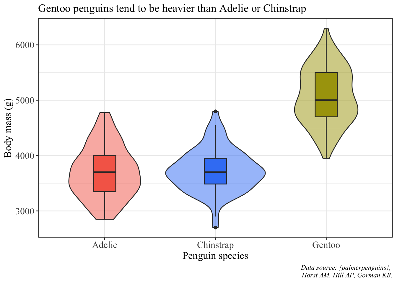
The plots above use the regular settings in ggplot, which is fine, but not exactly aesthetically pleasing. Remember that a big part of data science is data storytelling using visuals, and making those visuals clear and compelling to anyone who looks at them.

In this class, you’ll be expected to turn in “finalized” figures. This means that, at the very least, your axes are labelled something meaningful (for example, “Body mass (g)” instead of body_mass_g). However, there is a lot more to “finalizing” a plot than the bare minimum. Check out the resource posted on Canvas for more examples, and minimum guidelines for plots you submit for assignments.

We’ll use the violin + boxplot example to make into a finalized version.

Code

ggplot(data = penguins, aes(x = species, y = body_mass_g)) +
  # fill the violin shape using the species column: every species has a different color
  # alpha argument: makes the violin shape more transparent (scale of 0 to 1)
  geom_violin(aes(fill = species), alpha = 0.5) +
  # fill the boxplot shape using the species column
  # make the boxplots narrower
  geom_boxplot(aes(fill = species), width = 0.2) +
  # specify the colors you want to use for each species
  scale_fill_manual(values = c("#F56A56", "#3D83F5", "#A9A20B")) +
  # relabel the axis titles, plot title, and caption
  labs(x = "Penguin species", y = "Body mass (g)",
       title = "Gentoo penguins tend to be heavier than Adelie or Chinstrap",
       caption = "Data source: {palmerpenguins}, \n Horst AM, Hill AP, Gorman KB.") +
  # themes built in to ggplot
  theme_bw() +
  # other theme adjustments
  theme(legend.position = "none", 
        axis.title = element_text(size = 13),
        axis.text = element_text(size = 12),
        plot.title = element_text(size = 14),
        plot.caption = element_text(face = "italic"),
        text = element_text(family = "Times New Roman"))

Warning: Removed 2 rows containing non-finite values (`stat_ydensity()`).

Warning: Removed 2 rows containing non-finite values (`stat_boxplot()`).

Another one as an example is a plot with the mean point and standard deviation bars and jittered points:

Code

ggplot() +
  # using two different data frames: penguins (raw data) and penguins_summary (mean and SD)
  # raw data are jittered
  geom_jitter(data = penguins, aes(x = species, y = body_mass_g, color = species), alpha = 0.4) +
  # summary data: mean is a point, bars are standard deviation
  geom_point(data = penguin_summary, aes(x = species, y = mean_body_mass, color = species), size = 5) +
  geom_errorbar(data = penguin_summary, aes(x = species, ymin = mean_body_mass - sd_body_mass, ymax = mean_body_mass + sd_body_mass, color = species), width = 0.2) +
  scale_color_manual(values = c("#F56A56", "#3D83F5", "#A9A20B")) +
  labs(x = "Penguin species", y = "Body mass (g)",
       title = "Gentoo penguins tend to be heavier than Adelie or Chinstrap",
       caption = "Data source: {palmerpenguins}, \n Horst AM, Hill AP, Gorman KB.") +
  theme_bw() +
  theme(legend.position = "none", 
        axis.title = element_text(size = 13),
        axis.text = element_text(size = 12),
        plot.title = element_text(size = 14),
        plot.caption = element_text(face = "italic"),
        text = element_text(family = "Times New Roman"))

Warning: Removed 2 rows containing missing values (`geom_point()`).

Note: there is always more tinkering you can do with a figure. The best way to figure out if you’re actually communicating any kind of point or summarizing the data in a succinct way is to show your figure to someone else. You are not the best judge of how well you’re communicating - other people are! In this class, I encourage you to share your figures with classmates, friends, anyone who you can trust to give you good feedback about 1) whether you’ve communicated your message and 2) whether your figure actually looks good.

Citation

BibTeX citation:

@online{bui2023,
  author = {Bui, An},
  title = {Coding Workshop: {Week} 3},
  date = {2023-04-19},
  url = {https://an-bui.github.io/ES-193DS-W23/workshop/workshop-03_2023-04-19.html},
  langid = {en}
}

For attribution, please cite this work as:

Bui, An. 2023. “Coding Workshop: Week 3.” April 19, 2023. https://an-bui.github.io/ES-193DS-W23/workshop/workshop-03_2023-04-19.html.

0. set up

1. Basic data exploration and summarizing

a. Review

b. New functions: count(), mutate(), case_when()

count()

mutate() + case_when()

2. Review: rendering (Quarto) and knitting (RMarkdown)

3. Review: how to use ggplot

4. Exploratory data visualization

i. box plots

ii. violin plots

iii. jitter plot

iv. points with bars

v. some combination of the above

violin plot with boxplot

boxplot with jittered points

4. Adjusting ggplot defaults

Citation

b. New functions: `count()`, `mutate()`, `case_when()`

`count()`

`mutate()` + `case_when()`

3. Review: how to use `ggplot`

4. Adjusting `ggplot` defaults