0. set up

Code

library(tidyverse)
library(lterdatasampler)

1. Data

What is the first step to working with data?

Code

str(hbr_maples)

tibble [359 × 11] (S3: tbl_df/tbl/data.frame)
 $ year               : num [1:359] 2003 2003 2003 2003 2003 ...
 $ watershed          : Factor w/ 2 levels "Reference","W1": 1 1 1 1 1 1 1 1 1 1 ...
 $ elevation          : Factor w/ 2 levels "Low","Mid": 1 1 1 1 1 1 1 1 1 1 ...
 $ transect           : Factor w/ 12 levels "R1","R2","R3",..: 1 1 1 1 1 1 1 1 1 1 ...
 $ sample             : Factor w/ 20 levels "1","2","3","4",..: 1 2 3 4 5 6 7 8 9 10 ...
 $ stem_length        : num [1:359] 86.9 114 83.5 68.1 72.1 77.7 85.5 81.6 92.9 59.6 ...
 $ leaf1area          : num [1:359] 13.84 14.57 12.45 9.97 6.84 ...
 $ leaf2area          : num [1:359] 12.13 15.27 9.73 10.07 5.48 ...
 $ leaf_dry_mass      : num [1:359] 0.0453 0.0476 0.0423 0.0397 0.0204 0.0317 0.0382 0.0179 0.0286 0.0125 ...
 $ stem_dry_mass      : num [1:359] 0.03 0.0338 0.0248 0.0194 0.018 0.0246 0.0316 0.015 0.0291 0.0149 ...
 $ corrected_leaf_area: num [1:359] 29.1 33 25.3 23.2 15.5 ...

Code

# use View(hbr_maples) in the console to see the data frame

Are there any missing observations?

Use install.packages("naniar") in the console before running the chunk below.

Code

library(naniar)

gg_miss_var(hbr_maples)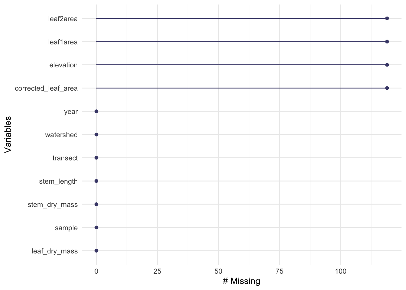

2. Do sugar maple stem lengths differ between reference and calcium-treated watersheds in 2003?

a. initial wrangling

Code

maples_2003 <- hbr_maples %>% 
  filter(year == 2003) %>% 
  mutate(watershed = case_when(
    watershed == "Reference" ~ "Reference", 
    watershed == "W1" ~ "Calcium-treated"
  ))

head(maples_2003, 5)

# A tibble: 5 × 11
   year watershed eleva…¹ trans…² sample stem_…³ leaf1…⁴ leaf2…⁵ leaf_…⁶ stem_…⁷
  <dbl> <chr>     <fct>   <fct>   <fct>    <dbl>   <dbl>   <dbl>   <dbl>   <dbl>
1  2003 Reference Low     R1      1         86.9   13.8    12.1   0.0453  0.03  
2  2003 Reference Low     R1      2        114     14.6    15.3   0.0476  0.0338
3  2003 Reference Low     R1      3         83.5   12.5     9.73  0.0423  0.0248
4  2003 Reference Low     R1      4         68.1    9.97   10.1   0.0397  0.0194
5  2003 Reference Low     R1      5         72.1    6.84    5.48  0.0204  0.018 
# … with 1 more variable: corrected_leaf_area <dbl>, and abbreviated variable
#   names ¹elevation, ²transect, ³stem_length, ⁴leaf1area, ⁵leaf2area,
#   ⁶leaf_dry_mass, ⁷stem_dry_mass

b. summary statistics

Remember, we’re interested in stem lengths in 2003 between reference and calcium-treated watersheds. What groups would be useful if that was the case?

Code

lengths_2003_summary <- maples_2003 %>% 
  group_by(watershed) %>% 
  summarize(mean_l = mean(stem_length),
            sd_l = sd(stem_length),
            var_l = var(stem_length),
            count_l = length(stem_length),
            se_l = sd_l/sqrt(count_l),
            margin_l = qt(0.95, df = count_l - 1) * se_l) 

lengths_2003_summary

# A tibble: 2 × 7
  watershed       mean_l  sd_l var_l count_l  se_l margin_l
  <chr>            <dbl> <dbl> <dbl>   <int> <dbl>    <dbl>
1 Calcium-treated   87.9  14.3  206.     120  1.31     2.17
2 Reference         81.0  13.9  194.     120  1.27     2.11

Code

# not getting the digits after the decimal point that you're expecting?
# try `as.data.frame()` piped in after the summarize call.

c. check for normally distributed data

Code

ggplot(data = maples_2003) +
  stat_qq(aes(sample = stem_length)) +
  stat_qq_line(aes(sample = stem_length), color = "red") +
  facet_wrap(~ watershed)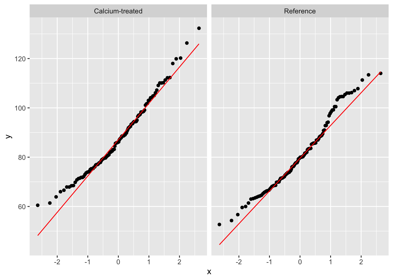

c. Check for equal variances

With an F-test, you can ask: are the sample variances between my two groups equal?
The assumption is that your data are normally distributed.

\[ H0: s^2_1 = s^2_2 H1: s^2_1 \neq s^2_2 \]

Code

length_var <- var.test(stem_length ~ watershed, data = maples_2003)

length_var


    F test to compare two variances

data:  stem_length by watershed
F = 1.0587, num df = 119, denom df = 119, p-value = 0.7563
alternative hypothesis: true ratio of variances is not equal to 1
95 percent confidence interval:
 0.7378244 1.5190473
sample estimates:
ratio of variances 
          1.058674

c. decide on a critical value

Two-tailed with significance level \(\alpha\) = 0.05:

Code

qt(p = .05/2, df = 119)

[1] -1.9801

If your test statistic is less than -1.98 or greater than 1.98, then you have evidence to reject the null hypothesis.

d. Do a t-test

Code

length_ttest <- t.test(stem_length ~ watershed, data = maples_2003, var.equal = TRUE)

length_ttest


    Two Sample t-test

data:  stem_length by watershed
t = 3.7797, df = 238, p-value = 0.0001985
alternative hypothesis: true difference in means between group Calcium-treated and group Reference is not equal to 0
95 percent confidence interval:
  3.304134 10.497532
sample estimates:
mean in group Calcium-treated       mean in group Reference 
                     87.88583                      80.98500

e. Calculate Cohen’s d effect size

Cohen’s d is a measure of how many standard deviations apart the two sample means are.

\[ Cohen's d = \frac{\bar{x_1} - \bar{x_2}}{\sqrt{(s^2_1 + s^2_2)/2}} \]

Note that you are using sample means in the numerator and sample variances in the denominator.

We can calculate this by hand (use install.packages("data.table") in the console before running the chunk below):

Code

library(data.table)

# create a data frame in data table format from lengths_2003_summary
lengths_dt <- setDT(lengths_2003_summary)

# pull out mean and variance values from the data table 
mean_ref_2003 <- lengths_dt[watershed == "Reference", mean_l]
mean_w1_2003 <- lengths_dt[watershed == "Calcium-treated", mean_l]
var_ref_2003 <- lengths_dt[watershed == "Reference", var_l]
var_w1_2003 <- lengths_dt[watershed == "Calcium-treated", var_l]

# calculate Cohen's d
d_byhand <- (mean_w1_2003 - mean_ref_2003) / sqrt((var_w1_2003 + var_ref_2003)/2)
d_byhand

[1] 0.4879597

Or using a function in a package:

Use install.packages("effsize") in the console before running the chunk below.

Code

library(effsize)

d_effsize <- cohen.d(stem_length ~ watershed, data = maples_2003)

Compare the two calculations:

Code

d_byhand

[1] 0.4879597

Code

d_effsize


Cohen's d

d estimate: 0.4879597 (small)
95 percent confidence interval:
    lower     upper 
0.2298792 0.7460402

make a plot

Code

ggplot(data = lengths_2003_summary, aes(x = watershed, y = mean_l, color = watershed)) +
  geom_point(size = 3) +
  geom_linerange(aes(ymin = mean_l - margin_l, ymax = mean_l + margin_l), linewidth = 1) +
  geom_jitter(data = maples_2003, aes(x = watershed, y = stem_length), alpha = 0.3) +
  scale_color_manual(values = c("Reference" = "#E57B33", "Calcium-treated" = "#039199")) +
  labs(x = "Watershed", y = "Stem length (mm)") +
  theme_classic() +
  theme(legend.position = "none",
        text = element_text(family = "Times New Roman"),
        axis.title = element_text(size = 14),
        axis.text = element_text(size = 12),
        plot.caption = element_text(hjust = 0),
        plot.caption.position = "plot",
        plot.title.position = "plot")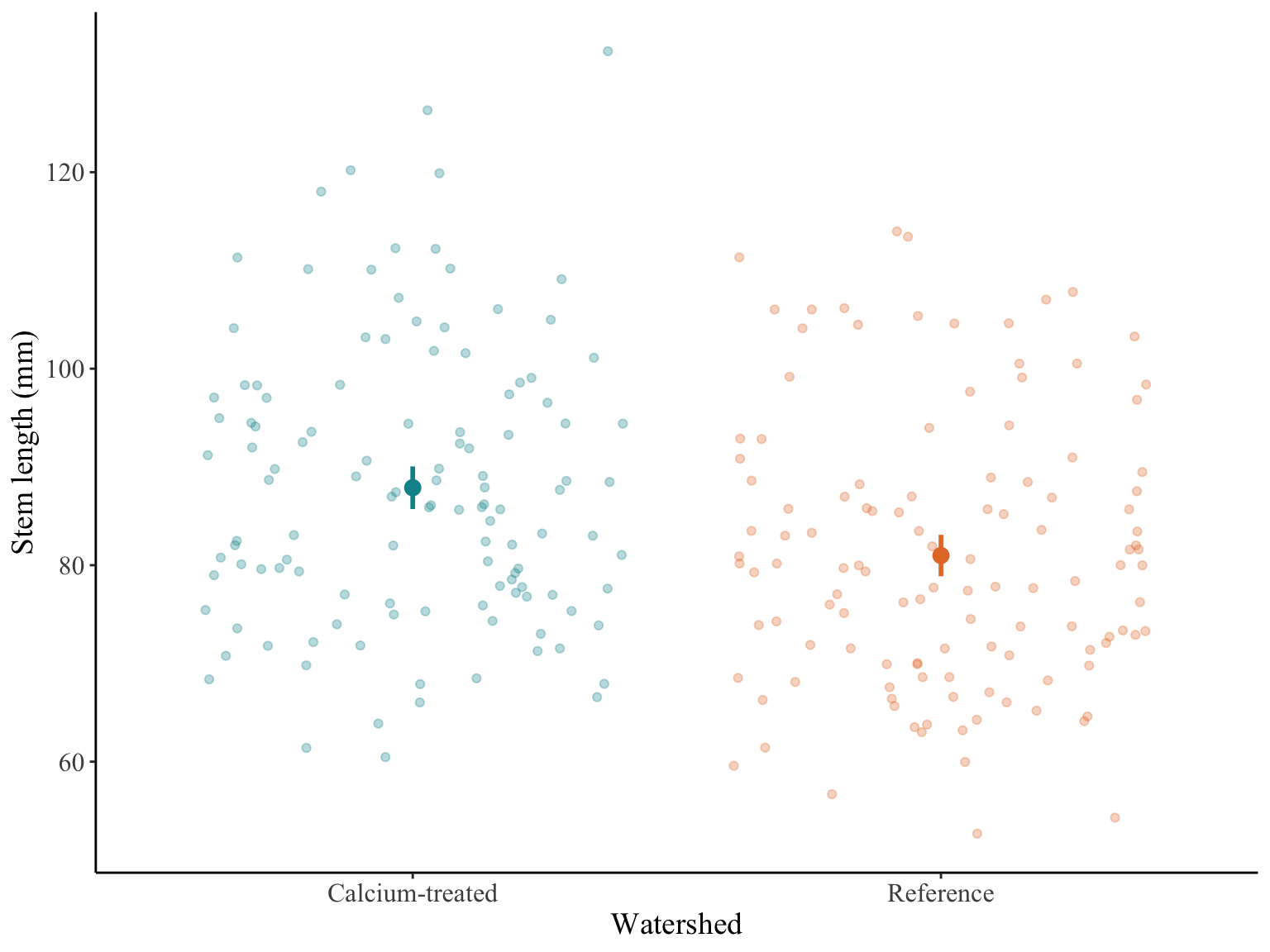

f. Communicating about the results of a t-test

figure caption

Figure 1. Sugar maple stem lengths in calcium-treated and reference watersheds. Stem lengths (mm) for calcium-treated (turquoise) and reference (orange) watersheds from Hubbard Brook Long-term Ecological Research site (HBR LTER). Dark points represent mean stem length and vertical lines represent confidence intervals with a 95% confidence level. Transparent points represent stem lengths.

in-text references

There is a moderate (Cohen’s d = 0.49) but significant effect of calcium treatment on sugar maple stem lengths (Student’s t-test, t(238) = 3.78, p < 0.001, \(\alpha\) = 0.05). On average, sugar maple stem lengths in calcium-treated watersheds were 6.9 mm longer than those in reference watersheds (95% confidence interval: [3.3, 10.5] mm, Figure 1).

bonus in-text references, using in-line R

When rendering your document, compare the text above with the text below. Are there any differences?

There is a moderate (Cohen’s d = 0.49) but significant effect of calcium treatment on sugar maple stem lengths (Student’s t-test, t(238) = 3.8, p < 0.001, \(\alpha\) = 0.05). On average, sugar maple stem lengths in calcium-treated watersheds were 6.9 mm longer than those in reference watersheds (CI = [3.3, 10.5] mm, Figure 1).

Citation

BibTeX citation:

@online{bui2023,
  author = {Bui, An},
  title = {Coding Workshop: {Week} 4},
  date = {2023-04-26},
  url = {https://an-bui.github.io/ES-193DS-W23/workshop/workshop-04_2023-04-26.html},
  langid = {en}
}

For attribution, please cite this work as:

Bui, An. 2023. “Coding Workshop: Week 4.” April 26, 2023. https://an-bui.github.io/ES-193DS-W23/workshop/workshop-04_2023-04-26.html.