Set up

Code

# should haves
library(tidyverse)
library(here)
library(lterdatasampler)

# would be nice to have
library(performance)
library(broom)
library(flextable)
library(ggeffects)
library(car)

1. Linear models

How does stem length predict stem dry mass?

Code

maples_data <- hbr_maples %>% 
  filter(year == 2003 & watershed == "Reference")

Look at your data (we’ve looked at this data set before, so we won’t go through it now)

Then, create some exploratory data visualization:

Code

ggplot(data = maples_data, aes(x = stem_length, y = stem_dry_mass)) +
  geom_point()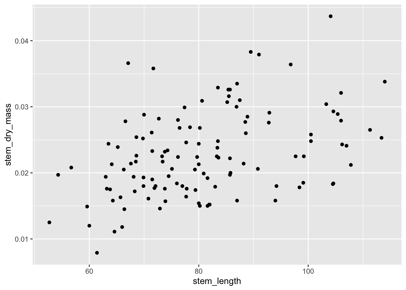

Seems like there should be a relationship between dry mass and length! Let’s try a model:

Code

modelobject <- lm(stem_dry_mass ~ stem_length, data = maples_data)

Code

# makes the viewer pane show a 2x2 grid of plots
# format: par(mfrow = c(number of rows, number of columns))
par(mfrow = c(2, 2))
plot(modelobject)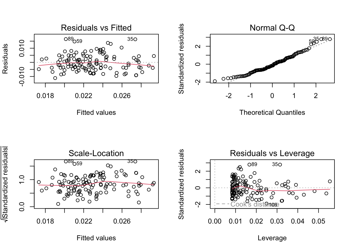

Code

# turns off the 2x2 grid - pop this under the code chunk where you set the 2x2 grid
dev.off()

2. Putting things together to communicate

a. model predictions

Code

# extract model predictions using ggpredict
predictions <- ggpredict(modelobject, terms = "stem_length")

predictions

# Predicted values of stem_dry_mass

stem_length | Predicted |       95% CI
--------------------------------------
         50 |      0.02 | [0.01, 0.02]
         60 |      0.02 | [0.02, 0.02]
         70 |      0.02 | [0.02, 0.02]
         80 |      0.02 | [0.02, 0.02]
         90 |      0.02 | [0.02, 0.03]
        100 |      0.03 | [0.02, 0.03]
        110 |      0.03 | [0.03, 0.03]
        120 |      0.03 | [0.03, 0.03]

Code

plot_predictions <- ggplot(data = maples_data, 
                           aes(x = stem_length, y = stem_dry_mass)) +
  # first plot the underlying data from maples_data
  geom_point() +
  # then plot the predictions
  geom_line(data = predictions, 
            aes(x = x, y = predicted), 
            color = "blue", linewidth = 1) +
  # then plot the 95% confidence interval from ggpredict
  geom_ribbon(data = predictions, 
              aes(x = x, y = predicted, ymin = conf.low, ymax = conf.high), 
              alpha = 0.2) +
  # theme and meaningful labels
  theme_bw() +
  labs(x = "Stem length (mm)",
       y = "Stem dry mass (g)")

plot_predictions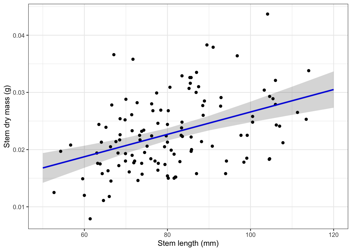

b. summary tables

Code

# store the model summary as an object
model_summary <- summary(modelobject)

# store the ANOVA table as an object
# anova(): special function to get analysis of variance tables for a model
model_squares <- anova(modelobject)

model_summary


Call:
lm(formula = stem_dry_mass ~ stem_length, data = maples_data)

Residuals:
       Min         1Q     Median         3Q        Max 
-0.0111253 -0.0039117 -0.0009091  0.0040911  0.0164587 

Coefficients:
             Estimate Std. Error t value Pr(>|t|)    
(Intercept) 7.003e-03  3.212e-03   2.180   0.0312 *  
stem_length 1.958e-04  3.909e-05   5.009 1.94e-06 ***
---
Signif. codes:  0 '***' 0.001 '**' 0.01 '*' 0.05 '.' 0.1 ' ' 1

Residual standard error: 0.005944 on 118 degrees of freedom
Multiple R-squared:  0.1753,    Adjusted R-squared:  0.1683 
F-statistic: 25.09 on 1 and 118 DF,  p-value: 1.94e-06

Code

model_squares

Analysis of Variance Table

Response: stem_dry_mass
             Df    Sum Sq    Mean Sq F value   Pr(>F)    
stem_length   1 0.0008864 0.00088642  25.089 1.94e-06 ***
Residuals   118 0.0041691 0.00003533                     
---
Signif. codes:  0 '***' 0.001 '**' 0.01 '*' 0.05 '.' 0.1 ' ' 1

model summary table:

Code

# don't name this chunk! some intricacies with Quarto: do not name chunks with tables in them

model_squares_table <- tidy(model_squares) %>% 
  # round the sum of squares and mean squares columns to have 5 digits (could be less)
  mutate(across(sumsq:meansq, ~ round(.x, digits = 5))) %>% 
  # round the F-statistic to have 1 digit
  mutate(statistic = round(statistic, digits = 1)) %>% 
  # replace the very very very small p value with < 0.001
  mutate(p.value = case_when(
    p.value < 0.001 ~ "< 0.001"
  )) %>% 
  # rename the stem_length cell to be meaningful
  mutate(term = case_when(
    term == "stem_length" ~ "Stem length (mm)",
    TRUE ~ term
  )) %>% 
  # make the data frame a flextable object
  flextable() %>% 
  # change the header labels to be meaningful
  set_header_labels(df = "Degrees of Freedom", 
                    sumsq = "Sum of squares",
                    meansq = "Mean squares",
                    statistic = "F-statistic",
                    p.value = "p-value")

model_squares_table

term	Degrees of Freedom	Sum of squares	Mean squares	F-statistic	p-value
Stem length (mm)	1	0.00089	0.00089	25.1	< 0.001
Residuals	118	0.00417	0.00004

Note! We didn’t get to analysis of variance in workshop on Wednesday. We will do it next week.

3. Analysis of variance

Do coastal giant salamander lengths differ by units?

Code

sal <- and_vertebrates %>% 
  # filter for the species and unit type
  filter(species == "Coastal giant salamander", 
         unittype %in% c("C", "P", "SC")) %>% 
  # creating a new column with the full unit name
  mutate(unit_name = case_when(
    unittype == "C" ~ "cascade", 
    unittype == "P" ~ "pool", 
    unittype == "SC" ~ "channel"
  )) %>% 
  # transforming the length variable with a natural log
  mutate(tf = log(length_1_mm))

Code

naniar::gg_miss_var(sal, facet = unit_name)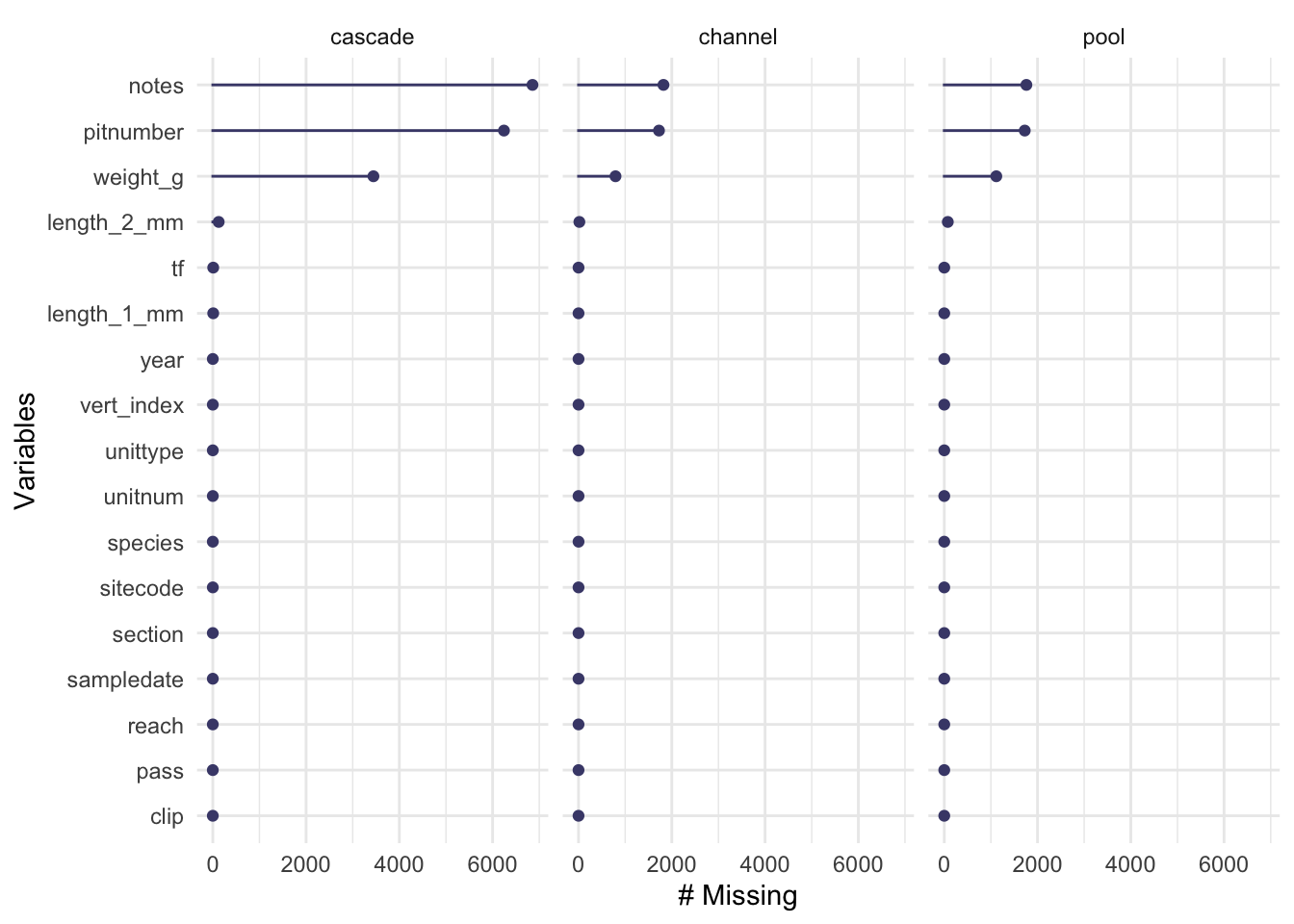

Code

sal_summary <- sal %>% 
  group_by(unit_name) %>% 
  summarize(mean = mean(length_1_mm, na.rm = TRUE),
            sd = sd(length_1_mm, na.rm = TRUE),
            count = length(length_1_mm), 
            se = sd/sqrt(count),
            var = var(length_1_mm, na.rm = TRUE))

sal_summary

# A tibble: 3 × 6
  unit_name  mean    sd count    se   var
  <chr>     <dbl> <dbl> <int> <dbl> <dbl>
1 cascade    58.3  20.8  7697 0.238  435.
2 channel    51.8  18.0  1994 0.403  324.
3 pool       57.3  22.8  1943 0.517  520.

Code

# if the largest sample variance is < 4× the smallest sample variance, the variances are close enough

Code

# weirdness with quarto: don't name code chunks if they have tables in them!

flextable(sal_summary) %>% 
  set_header_labels(unit_name = "Unit name",
                    mean = "Mean length (mm)", 
                    sd = "Standard deviation",
                    count = "Number of observations",
                    se = "Standard error",
                    var = "Variance")

Unit name	Mean length (mm)	Standard deviation	Number of observations	Standard error	Variance
cascade	58.31985	20.84792	7,697	0.2376304	434.6357
channel	51.77432	18.00636	1,994	0.4032398	324.2290
pool	57.28358	22.80015	1,943	0.5172510	519.8469

Code

ggplot(sal, aes(x = unit_name, y = length_1_mm)) +
  geom_boxplot()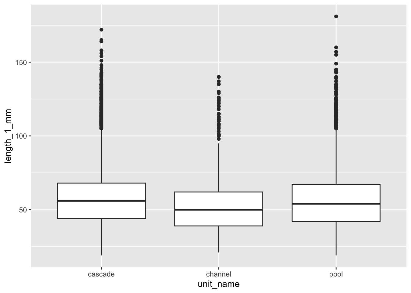

Code

ggplot(sal, aes(x = length_1_mm)) +
  geom_histogram() +
  facet_wrap(~ unit_name, scales = "free")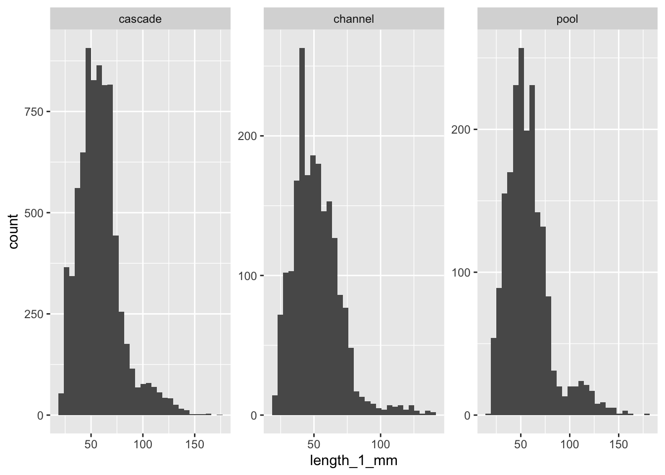

Code

ggplot(sal, aes(sample = length_1_mm)) +
  stat_qq_line(color = "blue") +
  stat_qq() +
  facet_wrap(~ unit_name)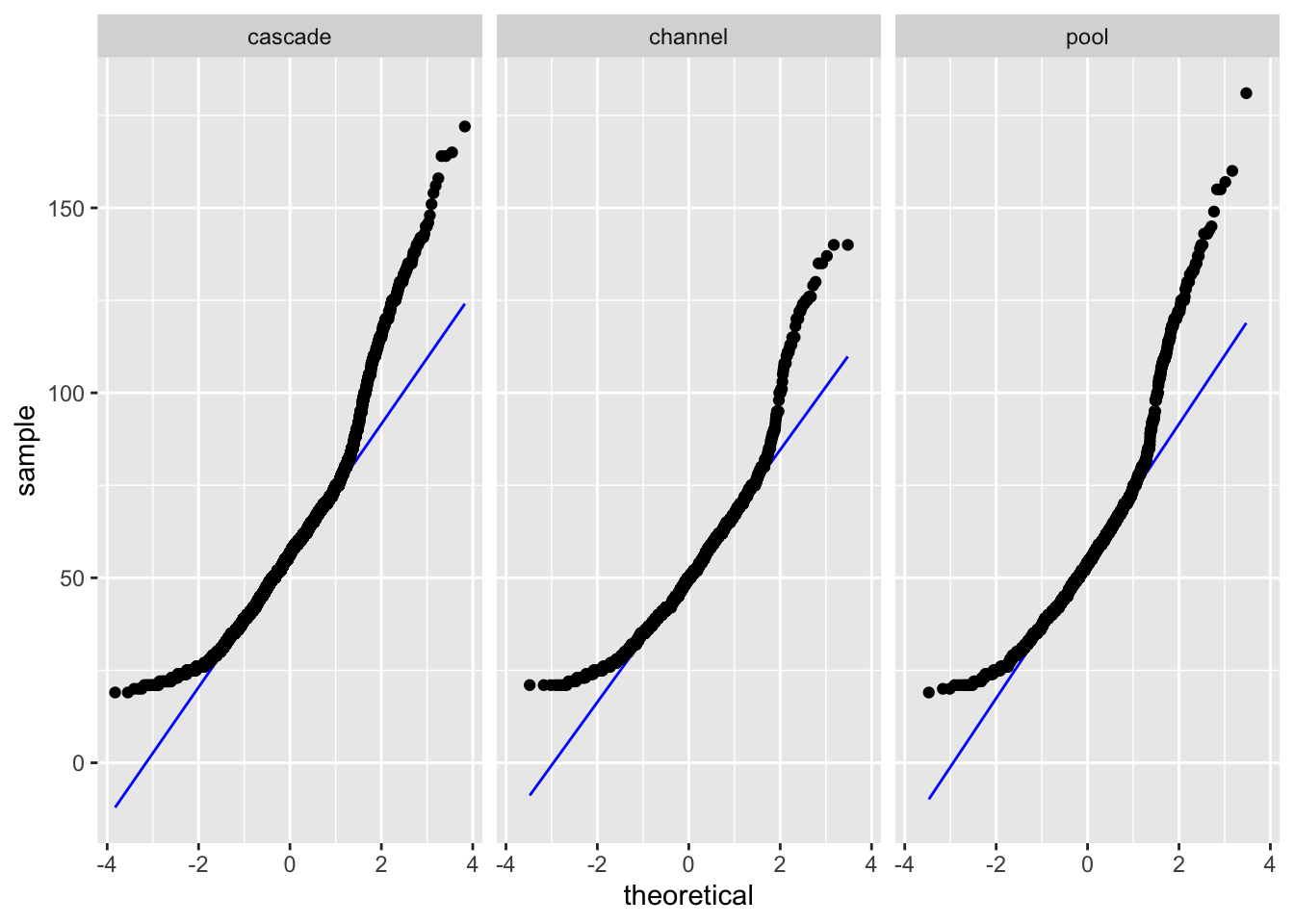

Code

leveneTest(length_1_mm ~ unit_name, data = sal)

Levene's Test for Homogeneity of Variance (center = median)
         Df F value    Pr(>F)    
group     2  20.922 8.516e-10 ***
      11622                      
---
Signif. codes:  0 '***' 0.001 '**' 0.01 '*' 0.05 '.' 0.1 ' ' 1

Code

# note different function from before!
sal_anova <- aov(length_1_mm ~ unit_name, data = sal)

summary(sal_anova)

               Df  Sum Sq Mean Sq F value Pr(>F)    
unit_name       2   67994   33997   79.07 <2e-16 ***
Residuals   11622 4996776     430                   
---
Signif. codes:  0 '***' 0.001 '**' 0.01 '*' 0.05 '.' 0.1 ' ' 1
9 observations deleted due to missingness

Code

TukeyHSD(sal_anova)

  Tukey multiple comparisons of means
    95% family-wise confidence level

Fit: aov(formula = length_1_mm ~ unit_name, data = sal)

$unit_name
                     diff       lwr        upr     p adj
channel-cascade -6.545526 -7.766976 -5.3240763 0.0000000
pool-cascade    -1.036267 -2.270380  0.1978461 0.1201769
pool-channel     5.509259  3.959921  7.0585969 0.0000000

tables:

Code

tidy(sal_anova)

# A tibble: 2 × 6
  term         df    sumsq meansq statistic   p.value
  <chr>     <dbl>    <dbl>  <dbl>     <dbl>     <dbl>
1 unit_name     2   67994. 33997.      79.1  7.77e-35
2 Residuals 11622 4996776.   430.      NA   NA

Transformations

(if we have time)

Code

ggplot(sal, aes(x = tf)) +
  geom_histogram() +
  facet_wrap(~ unit_name, scales = "free")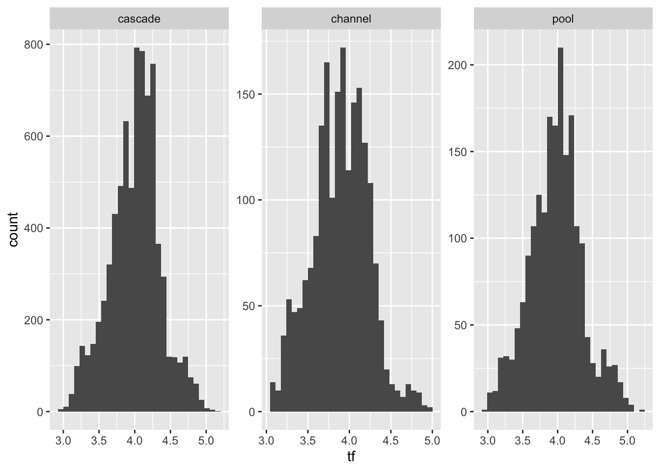

Code

ggplot(sal, aes(sample = tf)) +
  stat_qq_line(color = "blue") +
  stat_qq() +
  facet_wrap(~ unit_name)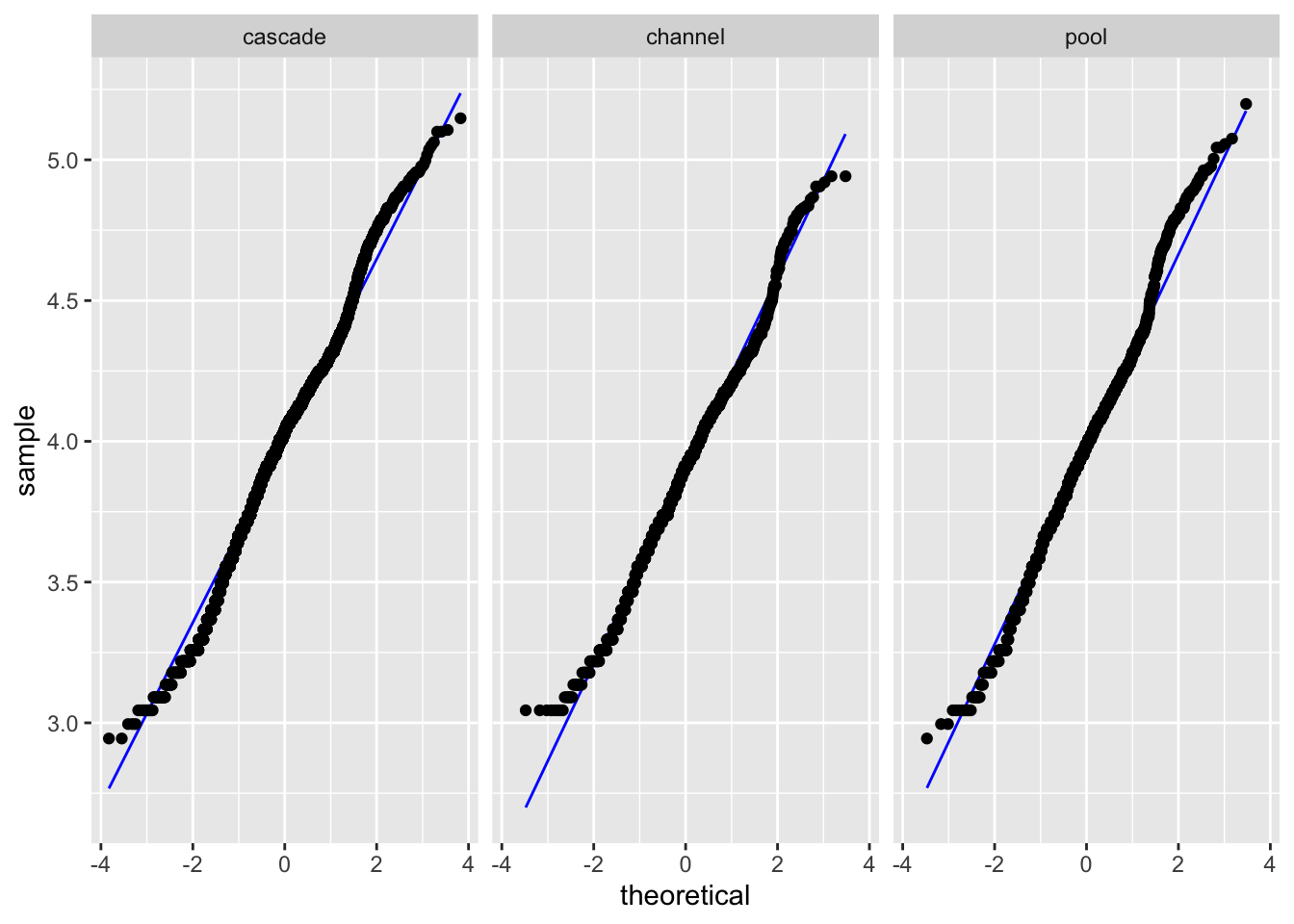

Code

leveneTest(tf ~ unit_name, data = sal)

Levene's Test for Homogeneity of Variance (center = median)
         Df F value   Pr(>F)   
group     2   6.103 0.002243 **
      11622                    
---
Signif. codes:  0 '***' 0.001 '**' 0.01 '*' 0.05 '.' 0.1 ' ' 1

Code

log_anova <- aov(tf ~ unit_name, data = sal)

par(mfrow = c(1, 2))
plot(log_anova, which = c(1))
plot(log_anova, which = c(2))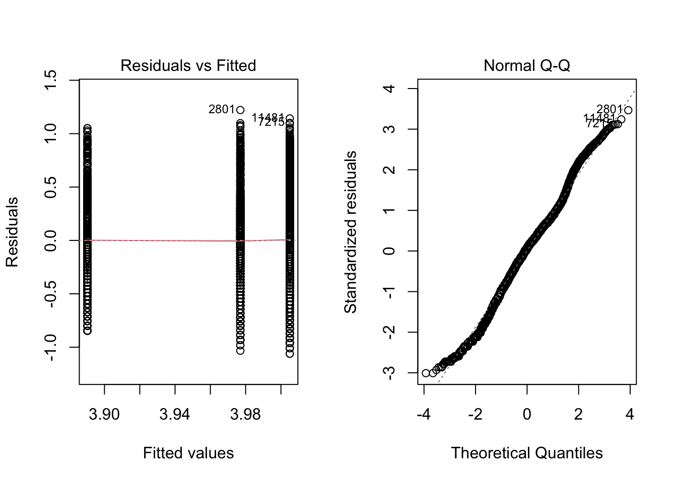

Code

dev.off()

Code

summary(log_anova)

               Df Sum Sq Mean Sq F value Pr(>F)    
unit_name       2   20.9  10.431   83.95 <2e-16 ***
Residuals   11622 1444.1   0.124                   
---
Signif. codes:  0 '***' 0.001 '**' 0.01 '*' 0.05 '.' 0.1 ' ' 1
9 observations deleted due to missingness

Code

TukeyHSD(log_anova)

  Tukey multiple comparisons of means
    95% family-wise confidence level

Fit: aov(formula = tf ~ unit_name, data = sal)

$unit_name
                       diff         lwr          upr     p adj
channel-cascade -0.11470205 -0.13546713 -0.093936962 0.0000000
pool-cascade    -0.02803709 -0.04901746 -0.007056729 0.0049454
pool-channel     0.08666495  0.06032566  0.113004248 0.0000000

Citation

BibTeX citation:

@online{bui2023,
  author = {Bui, An},
  title = {Coding Workshop: {Week} 7},
  date = {2023-05-17},
  url = {https://an-bui.github.io/ES-193DS-W23/workshop/workshop-07_2023-05-17.html},
  langid = {en}
}

For attribution, please cite this work as:

Bui, An. 2023. “Coding Workshop: Week 7.” May 17, 2023. https://an-bui.github.io/ES-193DS-W23/workshop/workshop-07_2023-05-17.html.