Notes from workshop

YAML options for a quarto document

---
title: "Untitled"
format:
  html:
    toc: true
    toc-location: left
    code-fold: true
    theme: yeti
execute:
  message: false
  warning: false
---

YAML options for an RMarkdown document:

---
title: "Untitled"
format:
  html_document:
    toc: true
    toc-location: left
    code_folding: true
    theme: yeti
---

knitr set up options for an RMarkdown document:

Code

knitr::opts_chunk$set(echo = TRUE, message = FALSE, warning = FALSE)

Set up

Code

# should haves (from last week)
library(tidyverse)
library(here)
library(janitor)
library(ggeffects)
library(performance)
library(naniar) # or equivalent
library(flextable) # or equivalent
library(car)
library(broom)
# would be nice to have
library(corrplot)
library(AICcmodavg)
library(GGally)

Read in the data:

Code

plant <- read_csv(here("data", "knb-lter-hfr.109.18", "hf109-01-sarracenia.csv")) %>% 
  # make the column names cleaner
  clean_names() %>% 
  # selecting the columns of interest
  select(totmass, species, feedlevel, sla, chlorophyll, amass, num_lvs, num_phylls)

Visualize the missing data:

Code

gg_miss_var(plant)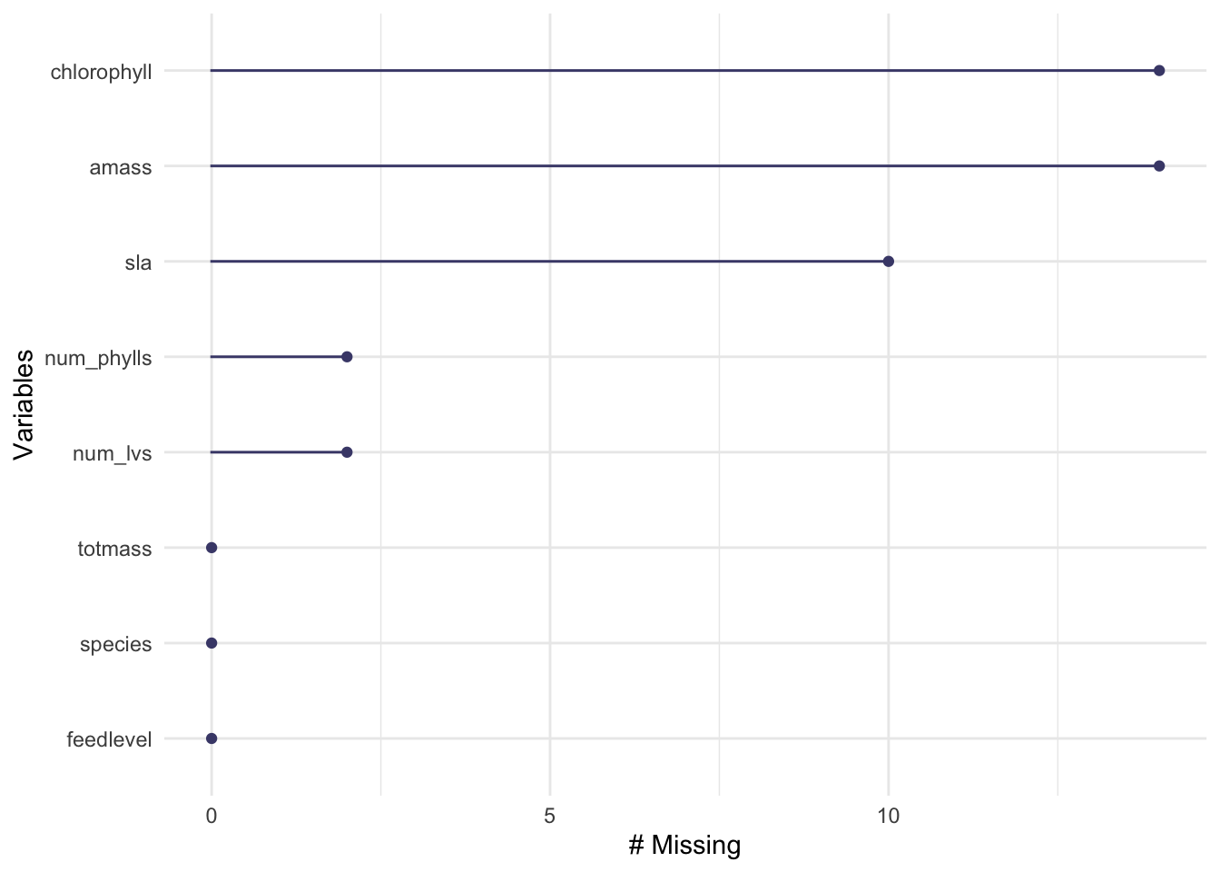

Subsetting the data by dropping NAs:

Code

plant_subset <- plant %>%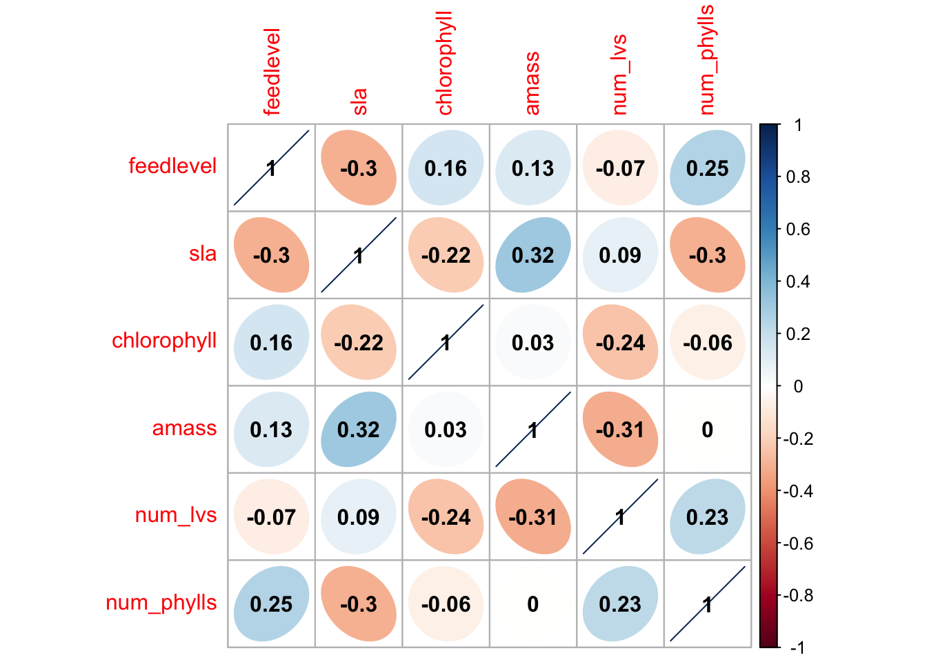 
  drop_na(sla, chlorophyll, amass, num_lvs, num_phylls)

Create a correlation plot:

(example writing) To determine the relationships between numerical variables in our dataset, we calculated Pearsons r and visually represented correlation using a correlation plot.

Code

# calculate Pearson's r for numerical values only
plant_cor <- plant_subset %>% 
  select(feedlevel:num_phylls) %>% 
  cor(method = "pearson")
  
# creating a correlation plot
corrplot(plant_cor,
         # change the shape of what's in the cells
         method = "ellipse",
         addCoef.col = "black"
         )

Create a plot of each varable compared against the others

Code

plant_subset %>% 
  select(species:num_phylls) %>% 
  ggpairs()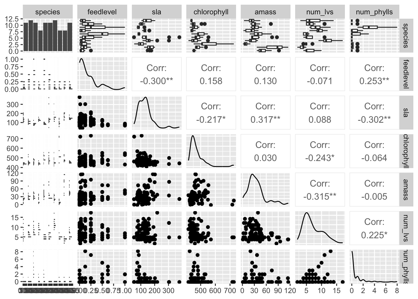

Starting regression here:

(example) To determine how species and physiological characteristics predict biomass, we fit multiple linear models.

Code

null <- lm(totmass ~ 1, data = plant_subset)
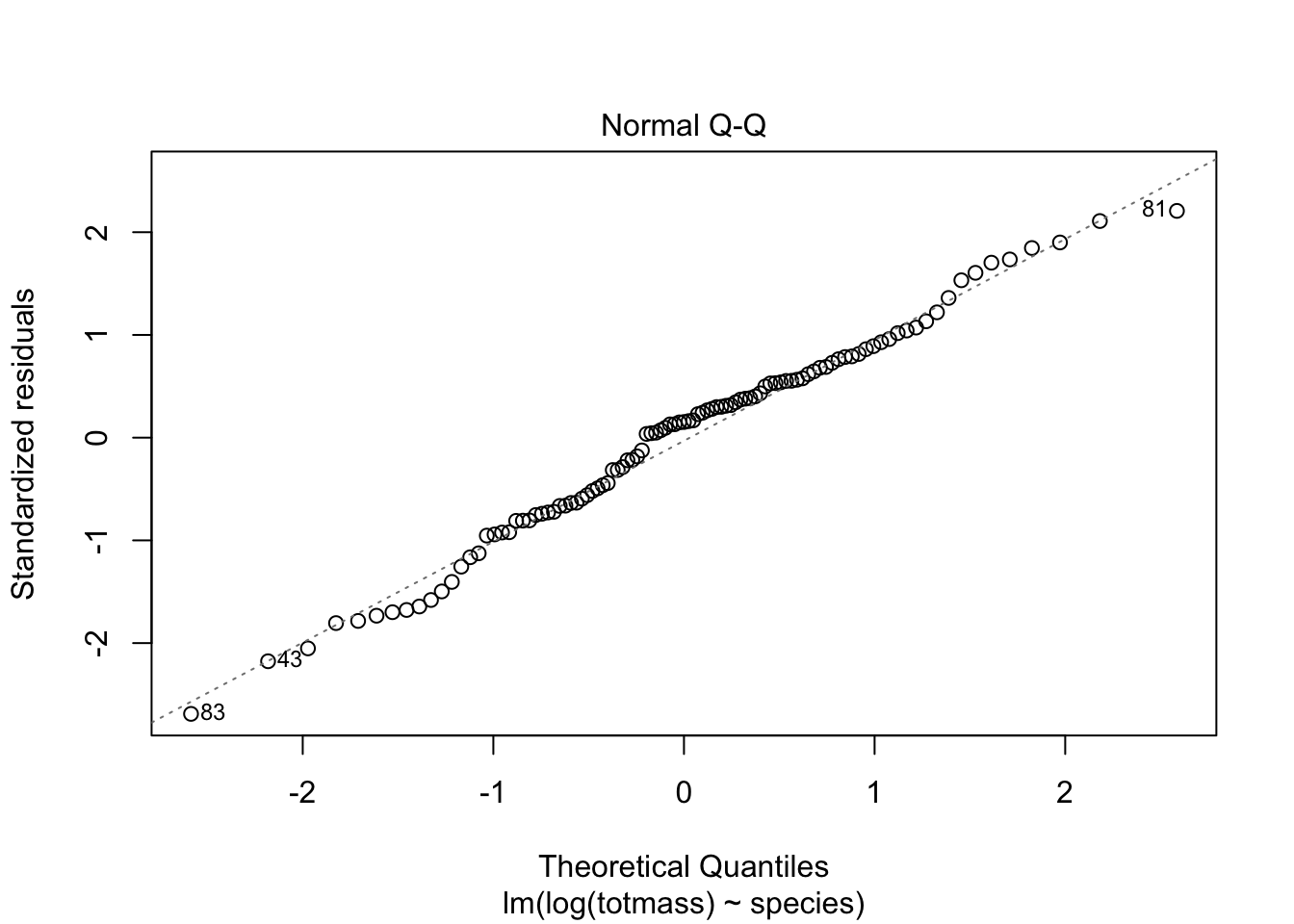
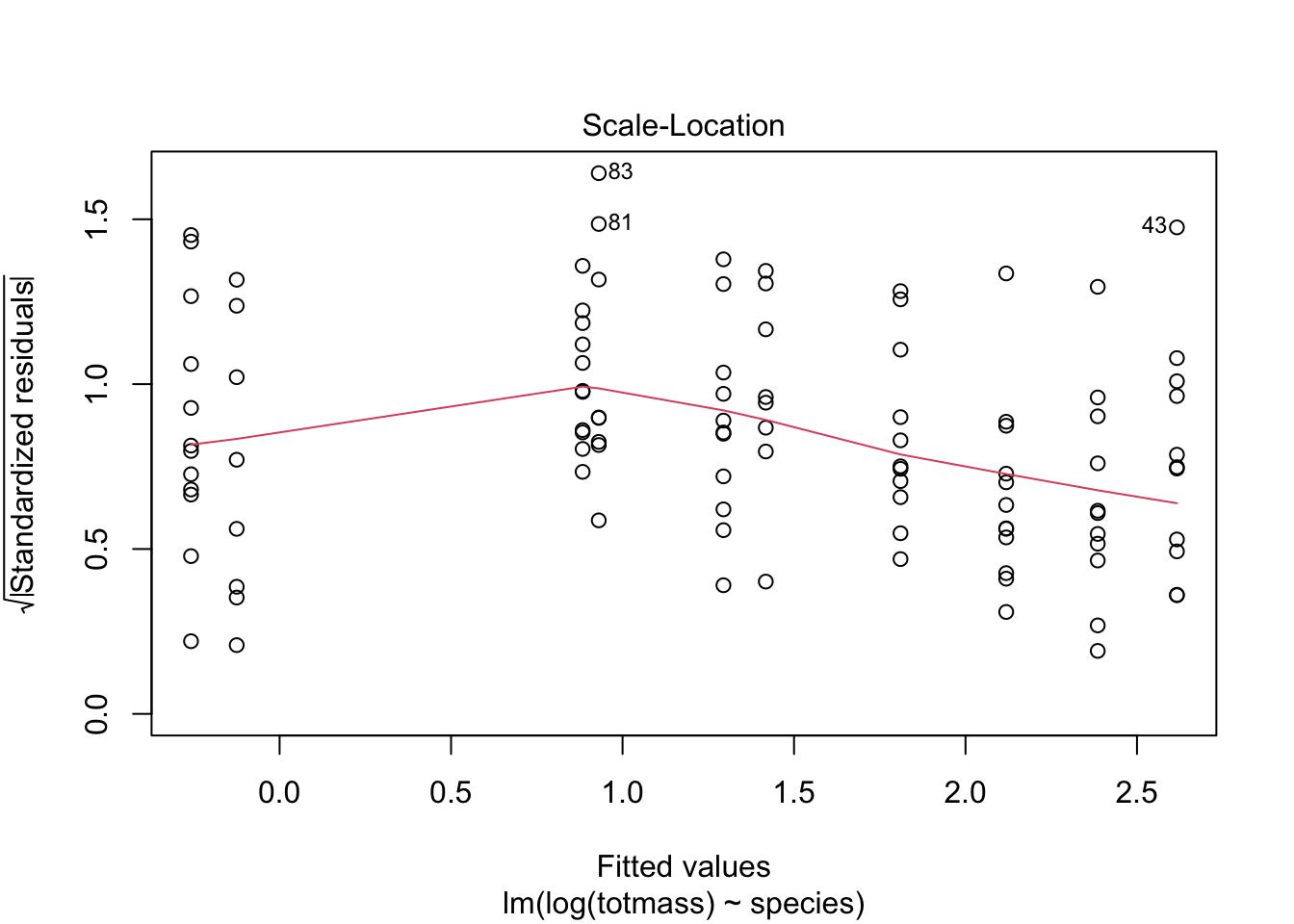
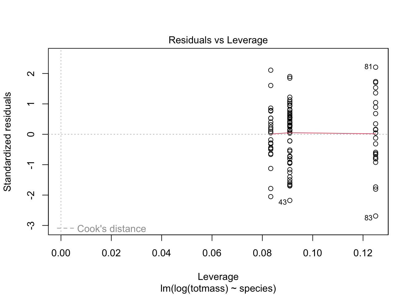
full <- lm(totmass ~ species + feedlevel + sla + chlorophyll + amass + num_lvs + num_phylls, data = plant_subset)

Diagnostics

We visually assess normality and homoskedasticity of residuals using diagnostic plots for the full model:

Code

par(mfrow = c(2, 2))
plot(full)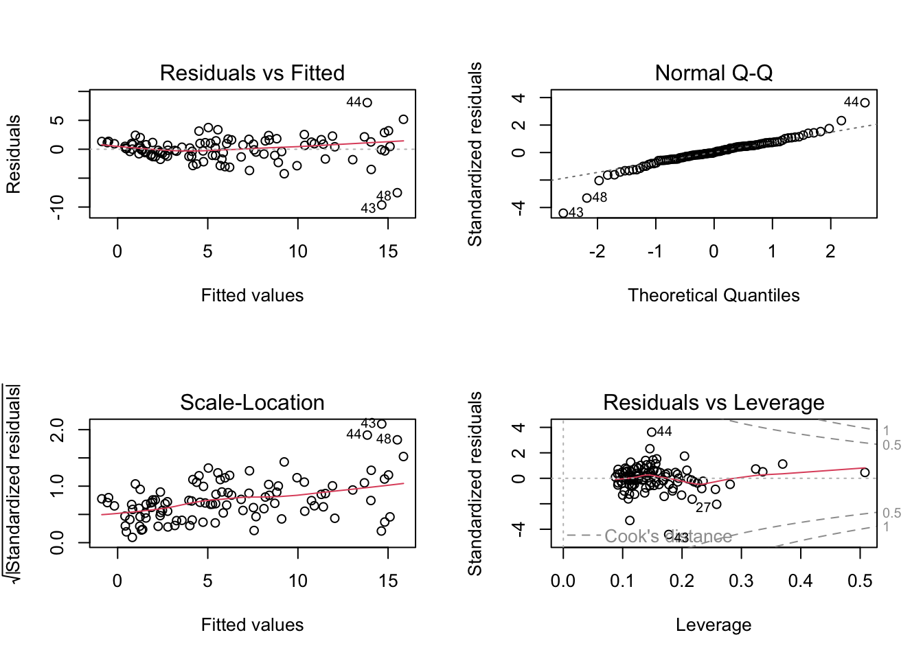

We also tested for normality using the Shapiro-Wilk test (null hypothesis: variable of interest (i.e. the residuals) are normally distributed).

We tested for heteroskedasticity using the Breusch-Pagan test (null hypothesis: variable of interest has constant variance).

Code

check_normality(full)

Warning: Non-normality of residuals detected (p < .001).

Code

check_heteroscedasticity(full)

Warning: Heteroscedasticity (non-constant error variance) detected (p < .001).

Code

null_log <- lm(log(totmass) ~ 1, data = plant_subset)
full_log <- lm(log(totmass) ~ species + feedlevel + sla + chlorophyll + amass + num_lvs + num_phylls, data = plant_subset)

plot(full_log)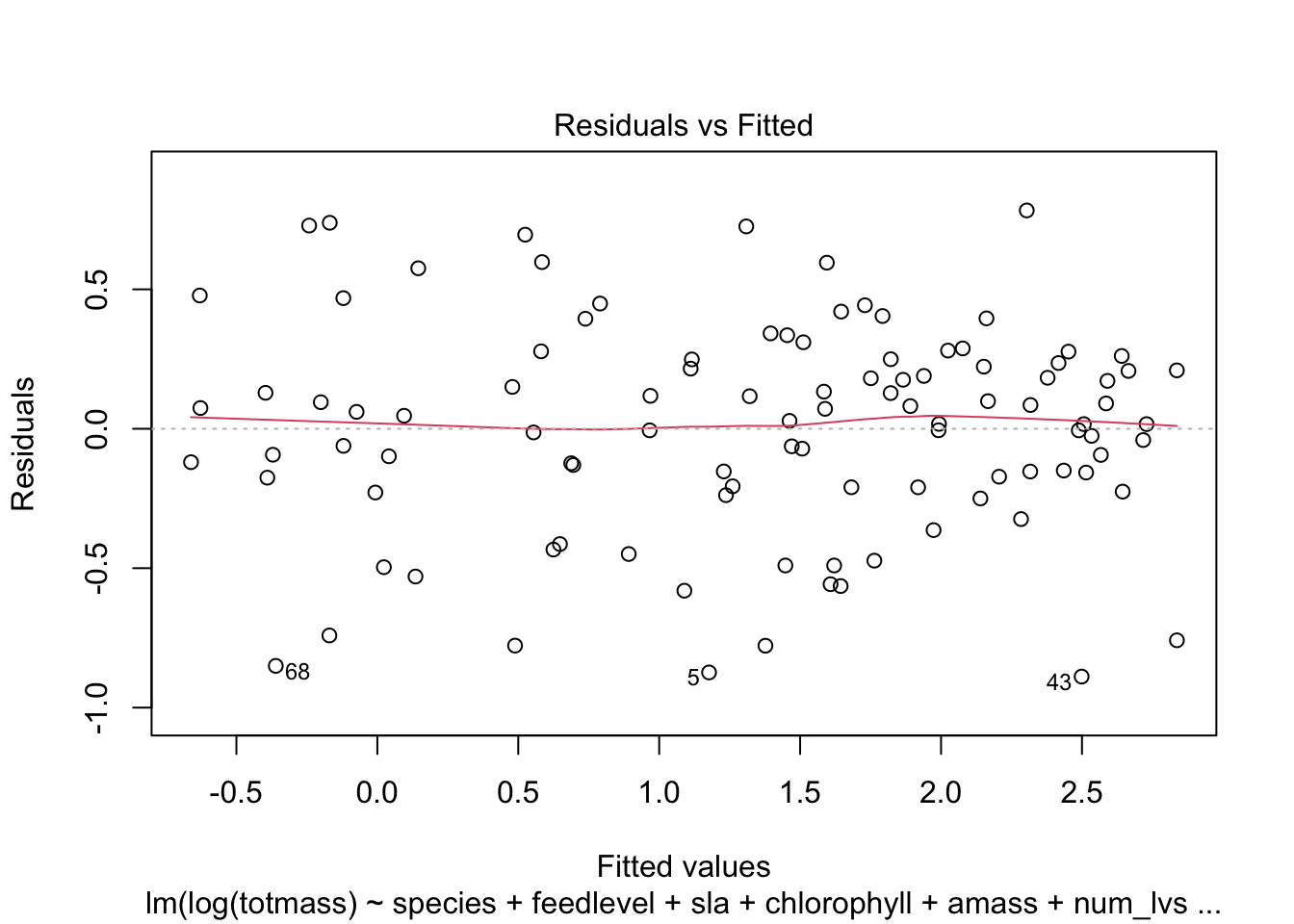

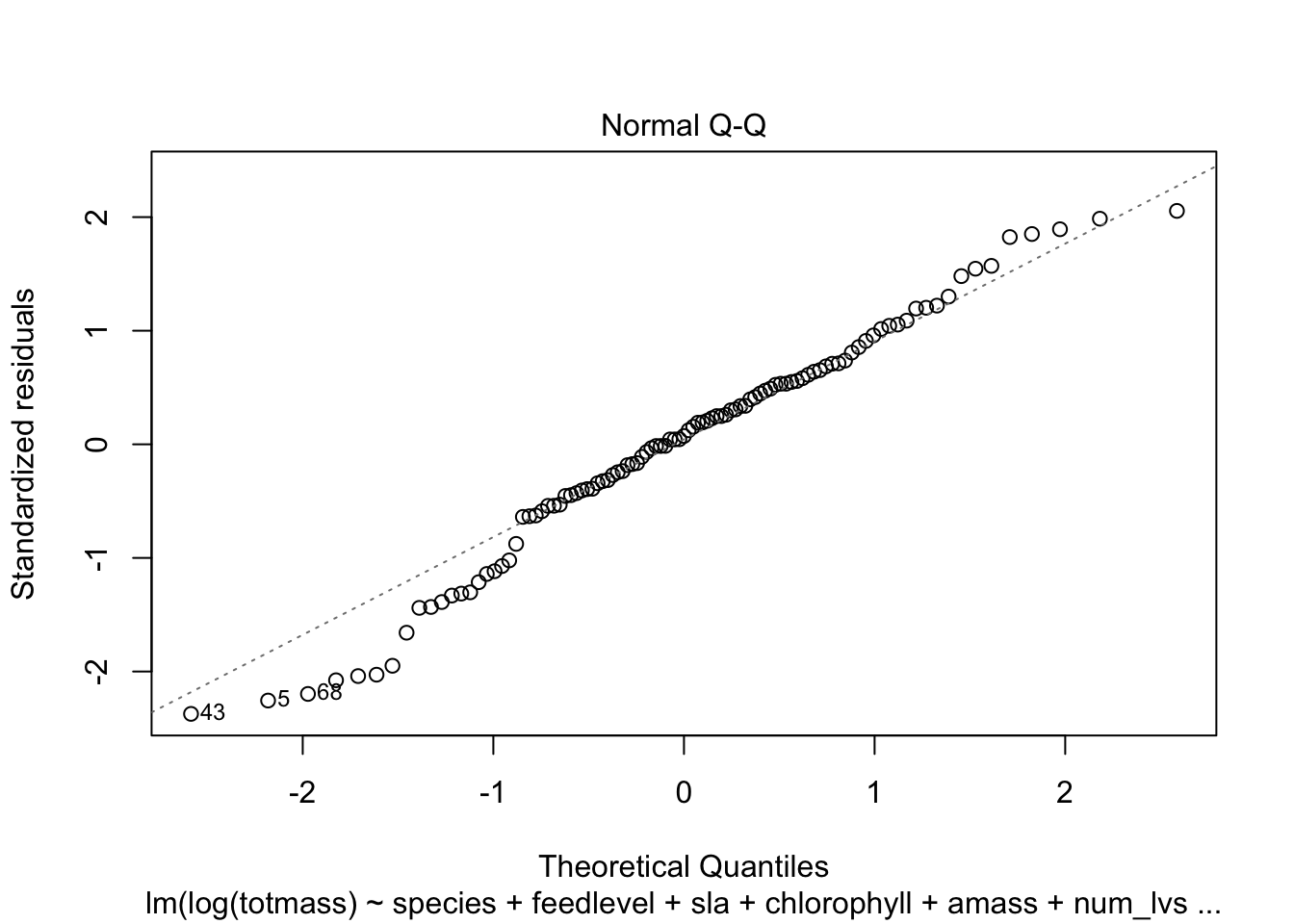
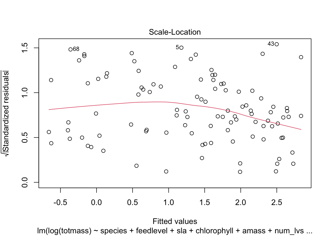
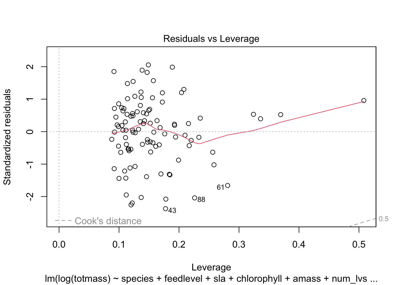
Code

check_normality(full_log)

OK: residuals appear as normally distributed (p = 0.107).

Code

check_heteroscedasticity(full_log)

OK: Error variance appears to be homoscedastic (p = 0.071).

Evaluate multicollinearity:

Code

car::vif(full_log)

                 GVIF Df GVIF^(1/(2*Df))
species     42.351675  9        1.231351
feedlevel    1.621993  1        1.273575
sla          1.999989  1        1.414210
chlorophyll  1.949828  1        1.396362
amass        2.872084  1        1.694722
num_lvs      2.813855  1        1.677455
num_phylls   2.995510  1        1.730754

We evaluated multicollinearity by calculating generalized variance inflation factor and determined that…

try some more models:

addressing the question: what set of predictor variables best explains the response?

Code

model2_log <- lm(log(totmass) ~ species, data = plant_subset)

check assumptions for model 2:

Code

plot(model2_log)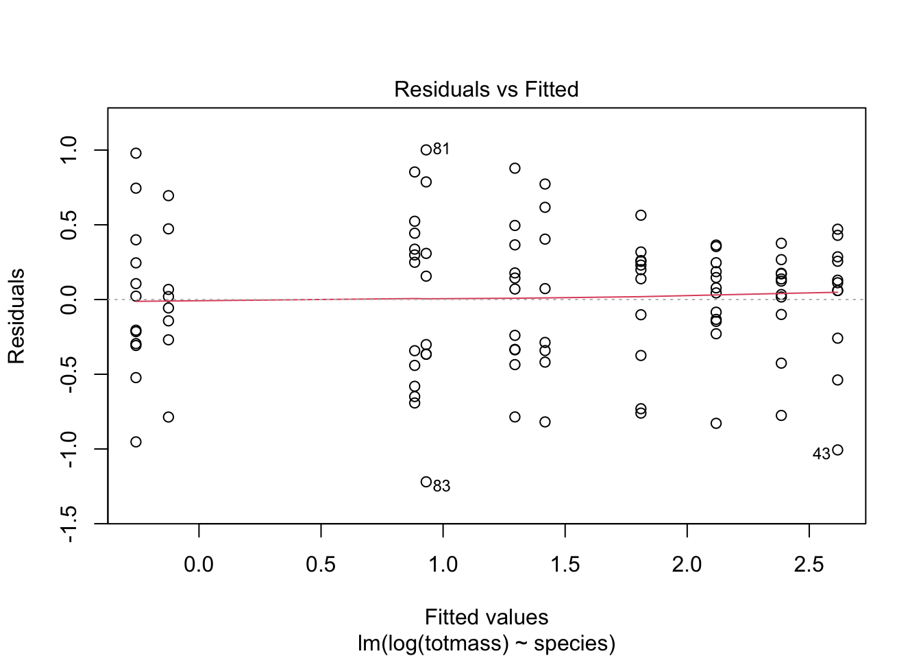

Code

check_normality(model2_log)

OK: residuals appear as normally distributed (p = 0.374).

Code

check_heteroscedasticity(model2_log)

OK: Error variance appears to be homoscedastic (p = 0.100).

compare models using Akaike’s Information criterion (AIC) values:

Code

AICc(full_log)

[1] 133.9424

Code

AICc(model2_log)

[1] 157.5751

Code

AICc(null_log)

[1] 306.0028

Code

MuMIn::AICc(full_log, model2_log, null_log)

           df     AICc
full_log   17 133.9424
model2_log 11 157.5751
null_log    2 306.0028

Code

MuMIn::model.sel(full_log, model2_log, null_log)

Model selection table 
             (Int)      ams      chl     fdl num_lvs  num_phy       sla spc df
full_log   -1.3390 0.002338 0.004368 -0.4743 0.09176 -0.03959 -0.002493   + 17
model2_log  0.8836                                                        + 11
null_log    1.3500                                                           2
             logLik  AICc  delta weight
full_log    -46.371 133.9   0.00      1
model2_log  -66.337 157.6  23.63      0
null_log   -150.941 306.0 172.06      0
Models ranked by AICc(x)

we compared models using AIC and chose the model with the lowest value, which was…

Results

We found that the ______ model including ___ ____ __ predictors best predicted _______ (model summary).

Code

summary(full_log)


Call:
lm(formula = log(totmass) ~ species + feedlevel + sla + chlorophyll + 
    amass + num_lvs + num_phylls, data = plant_subset)

Residuals:
     Min       1Q   Median       3Q      Max 
-0.88872 -0.20811  0.02825  0.24218  0.78287 

Coefficients:
                    Estimate Std. Error t value Pr(>|t|)    
(Intercept)        -1.339043   0.597727  -2.240 0.027624 *  
speciesalata        1.113163   0.184021   6.049 3.56e-08 ***
speciesflava        1.404562   0.262955   5.341 7.29e-07 ***
speciesjonesii      0.319652   0.196426   1.627 0.107281    
speciesleucophylla  1.709035   0.227608   7.509 4.88e-11 ***
speciesminor        0.389310   0.187903   2.072 0.041239 *  
speciespsittacina  -1.645198   0.207035  -7.946 6.36e-12 ***
speciespurpurea    -0.364348   0.254380  -1.432 0.155643    
speciesrosea       -0.947383   0.260495  -3.637 0.000467 ***
speciesrubra        0.875342   0.196361   4.458 2.46e-05 ***
feedlevel          -0.474255   0.234493  -2.022 0.046199 *  
sla                -0.002493   0.001160  -2.149 0.034430 *  
chlorophyll         0.004368   0.001189   3.672 0.000414 ***
amass               0.002338   0.002988   0.782 0.436166    
num_lvs             0.091764   0.022413   4.094 9.46e-05 ***
num_phylls         -0.039585   0.051714  -0.765 0.446068    
---
Signif. codes:  0 '***' 0.001 '**' 0.01 '*' 0.05 '.' 0.1 ' ' 1

Residual standard error: 0.413 on 87 degrees of freedom
Multiple R-squared:  0.8687,    Adjusted R-squared:  0.8461 
F-statistic: 38.38 on 15 and 87 DF,  p-value: < 2.2e-16

Code

table <- tidy(full_log, conf.int = TRUE) %>% 
  # change the p-value numbers if they're really small
  # change the estmaes, standard error, and t-tstatistics to round to ___ digits
  # using mutate
  # make it into a flextable
  flextable() %>% 
  # fit it to the viewer
  autofit()

table

term	estimate	std.error	statistic	p.value	conf.low	conf.high
(Intercept)	-1.339043200	0.597726532	-2.2402271	0.027624109607483092	-2.527089405	-0.1509969955
speciesalata	1.113162580	0.184020930	6.0491086	0.000000035633453091	0.747401056	1.4789241035
speciesflava	1.404562038	0.262954818	5.3414577	0.000000728606298866	0.881910865	1.9272132117
speciesjonesii	0.319652351	0.196426010	1.6273423	0.107280978897063603	-0.070765614	0.7100703152
speciesleucophylla	1.709035391	0.227608275	7.5086698	0.000000000048774953	1.256639298	2.1614314841
speciesminor	0.389310367	0.187903472	2.0718636	0.041239074384119417	0.015831871	0.7627888636
speciespsittacina	-1.645197874	0.207034720	-7.9464830	0.000000000006356134	-2.056701798	-1.2336939506
speciespurpurea	-0.364347584	0.254380246	-1.4322951	0.155642631385407848	-0.869955868	0.1412607001
speciesrosea	-0.947383285	0.260494896	-3.6368593	0.000466976667424191	-1.465145097	-0.4296214723
speciesrubra	0.875341885	0.196361315	4.4578123	0.000024573993550446	0.485052508	1.2656312619
feedlevel	-0.474255269	0.234492879	-2.0224719	0.046198841611705344	-0.940335257	-0.0081752817
sla	-0.002493083	0.001160230	-2.1487826	0.034429589763780327	-0.004799167	-0.0001869994
chlorophyll	0.004368330	0.001189484	3.6724575	0.000414110175835846	0.002004101	0.0067325586
amass	0.002337656	0.002988210	0.7822929	0.436166480376765642	-0.003601736	0.0082770479
num_lvs	0.091763935	0.022413350	4.0941643	0.000094562482452723	0.047214976	0.1363128941
num_phylls	-0.039585071	0.051713890	-0.7654630	0.446067519262092982	-0.142372027	0.0632018848

use ggpredict() to backtranform estimates

Code

model_pred <- ggpredict(full_log, terms = "species", back.transform = TRUE)

plot(ggpredict(full_log, terms = "species", back.transform = TRUE), add.data = TRUE)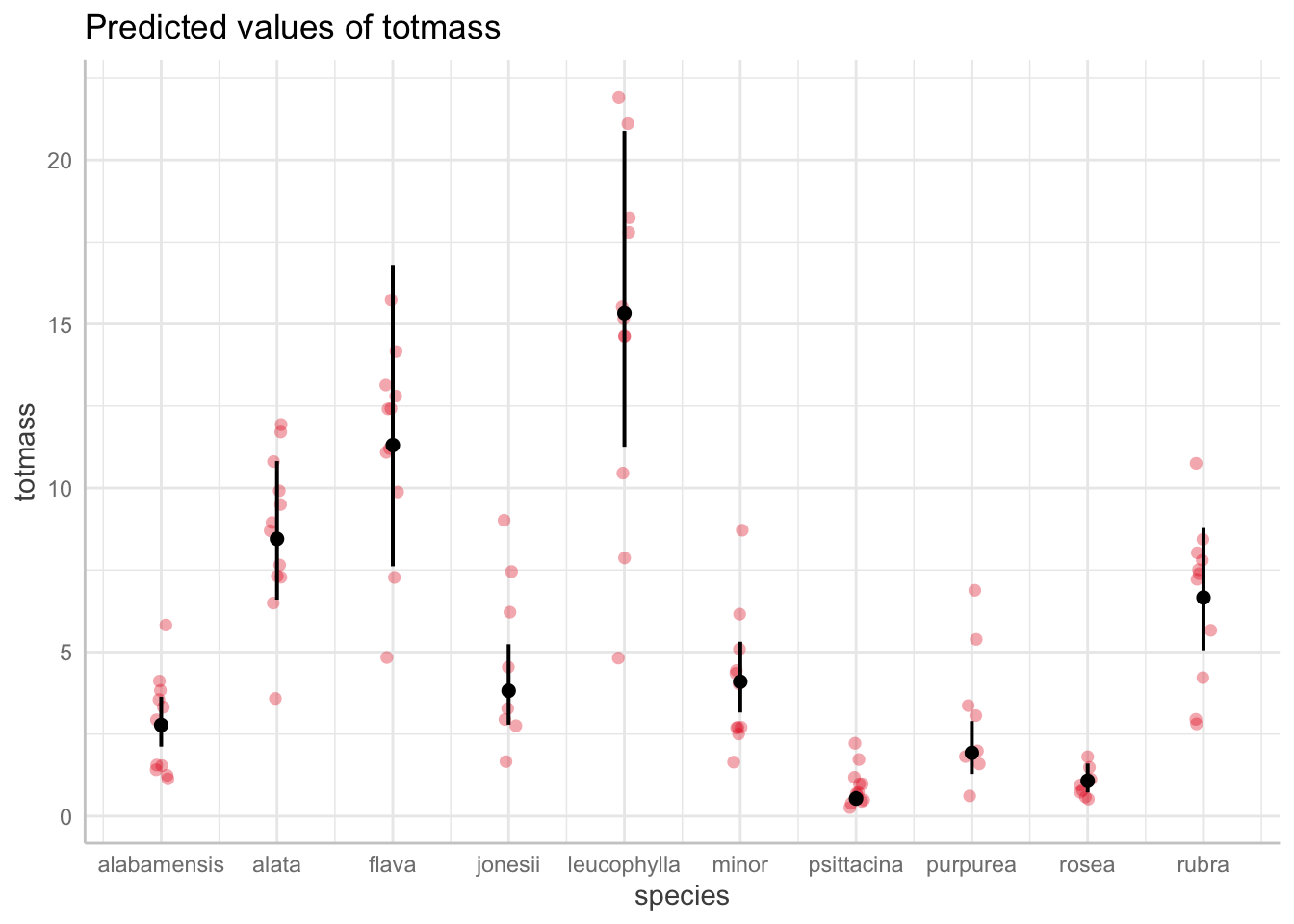

Code

plot(ggpredict(full_log, terms = "chlorophyll", back.transform = TRUE), add.data = TRUE)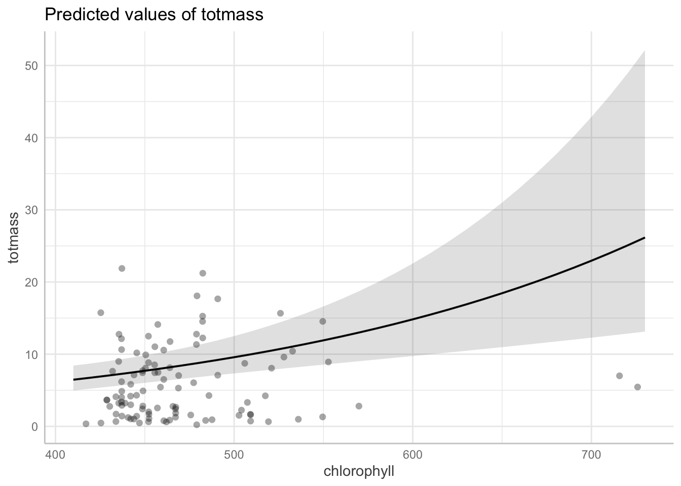

Code

plot(ggpredict(full_log, terms = "sla", back.transform = TRUE), add.data = TRUE)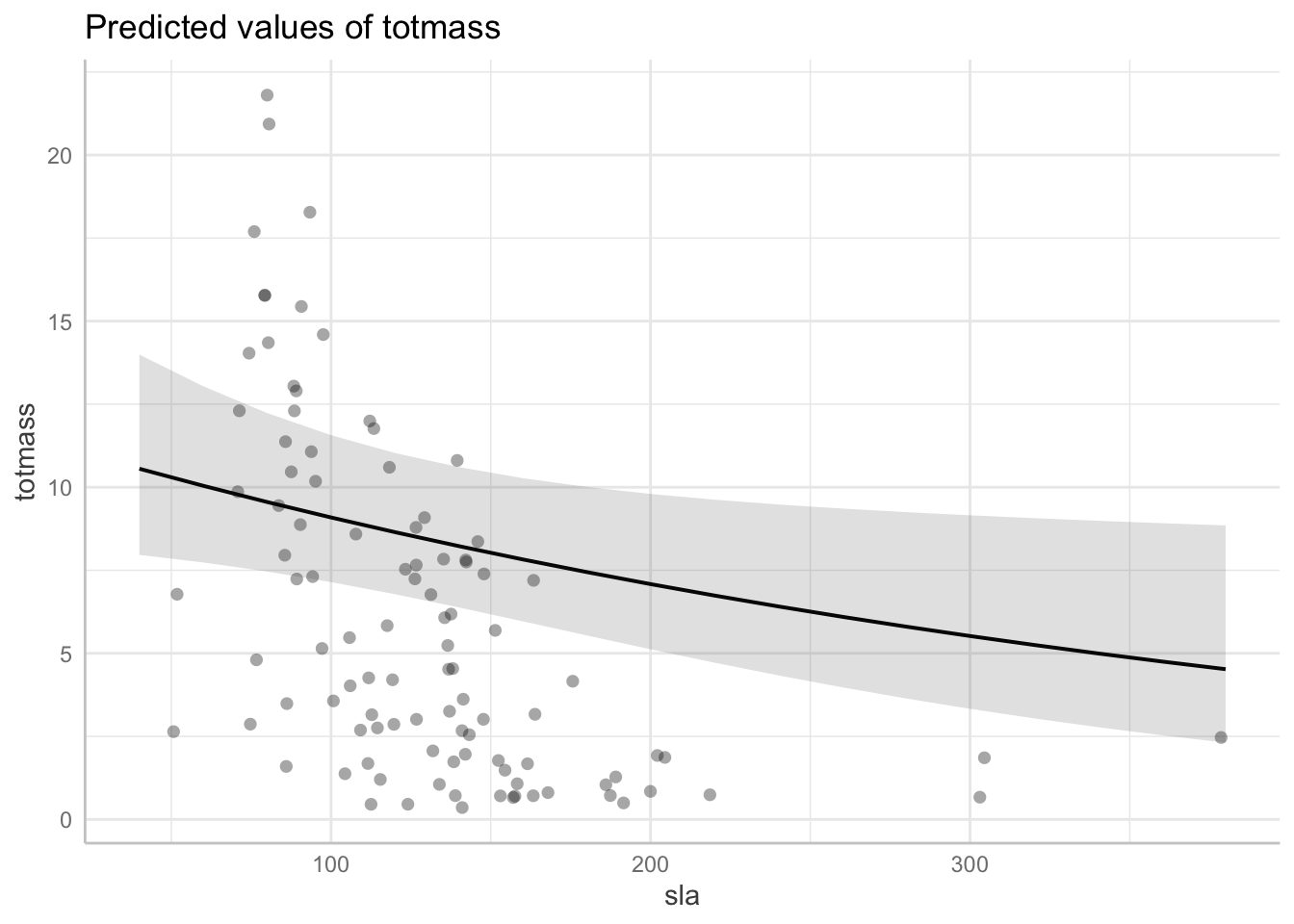

Code

model_pred

# Predicted values of totmass

species     | Predicted |        95% CI
---------------------------------------
alabamensis |      2.78 | [2.12,  3.64]
alata       |      8.45 | [6.60, 10.82]
flava       |     11.31 | [7.61, 16.80]
jonesii     |      3.82 | [2.79,  5.24]
minor       |      4.10 | [3.16,  5.31]
psittacina  |      0.54 | [0.37,  0.77]
purpurea    |      1.93 | [1.28,  2.90]
rubra       |      6.66 | [5.05,  8.78]

Adjusted for:
*   feedlevel =   0.18
*         sla = 129.27
* chlorophyll = 471.29
*       amass =  35.26
*     num_lvs =   7.08
*  num_phylls =   0.58

Citation

BibTeX citation:

@online{bui2023,
  author = {Bui, An},
  title = {Coding Workshop: {Week} 8 and 9},
  date = {2023-05-24},
  url = {https://an-bui.github.io/ES-193DS-W23/workshop/workshop-08_2023-05-24.html},
  langid = {en}
}

For attribution, please cite this work as:

Bui, An. 2023. “Coding Workshop: Week 8 and 9.” May 24, 2023. https://an-bui.github.io/ES-193DS-W23/workshop/workshop-08_2023-05-24.html.